The linear model with categorical predictors (ANOVA)
Last Updated: 21, November, 2024 at 09:18
library(reshape)
One way Anova: one categorical predictor
Fake data
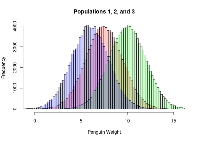
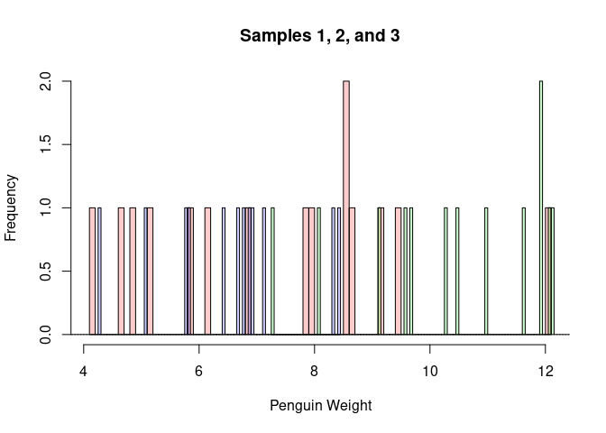
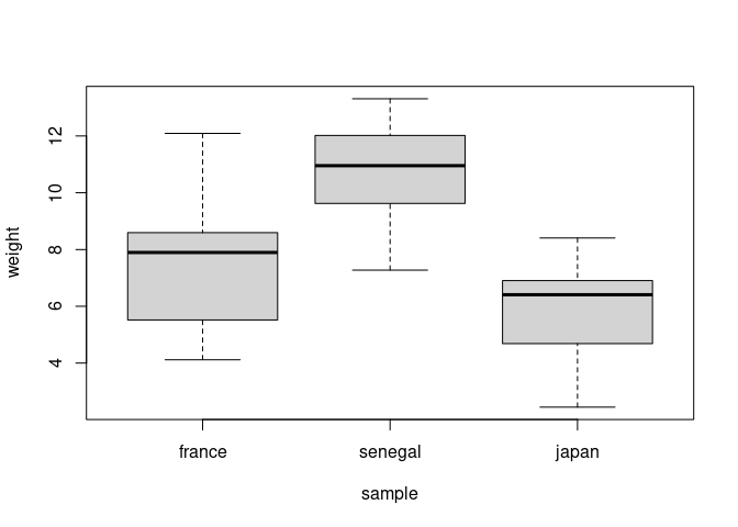
The data below is the same data as covered in the slides (fake data about three different penguin populations in France, Senegal, and Japan). The data is generated from three normal distributions with different means and standard deviations. The data is then sampled from these populations to create three samples of penguin weights.
For the purpose of learning to run ANOVA using the linear model, you can skio the code below and jump to the section on running the ANOVA.
### Make some population data
sample_size <- 15

population1 <- rnorm(100000, mean = 7.5, sd = 2)
population2 <- rnorm(100000, mean = 10, sd = 2)
population3 <- rnorm(100000, mean = 6, sd = 2)

hist(population1, breaks=100, col=rgb(1,0,0,0.2), main='', xlab = 'Penguin Weight')
hist(population2, breaks=100,  add=TRUE, col=rgb(0,1,0,0.2))
hist(population3, breaks=100,  add=TRUE, col=rgb(0,0,1,0.2))
title('Populations 1, 2, and 3')
Sample from the populations
france <- sample(population1, sample_size)
senegal <- sample(population2, sample_size)
japan <- sample(population3, sample_size)

hist(france, breaks=100, col=rgb(1,0,0,0.2), main='', xlab='Penguin Weight')
hist(senegal, breaks=100,  add=TRUE, col=rgb(0,1,0,0.2))
hist(japan, breaks=100,  add=TRUE, col=rgb(0,0,1,0.2))
title('Samples 1, 2, and 3')
data <-data.frame(cbind(france,senegal,japan))
data<-melt(data, id.vars=c())
colnames(data) <- c('sample', 'weight')
data$sample<-factor(data$sample)
head(data)
##   sample   weight
## 1 france 5.881672
## 2 france 8.522589
## 3 france 7.896305
## 4 france 4.661368
## 5 france 7.972789
## 6 france 6.167368
tail(data)
##    sample   weight
## 40  japan 6.409211
## 41  japan 5.763631
## 42  japan 8.335101
## 43  japan 2.936399
## 44  japan 6.670293
## 45  japan 6.914236
boxplot(weight ~ sample, data = data)
Run classic one-way ANOVA
result <- aov(weight ~ sample, data = data)
summary(result)
##             Df Sum Sq Mean Sq F value   Pr(>F)
## sample       2  192.1   96.04   25.34 6.05e-08 ***
## Residuals   42  159.2    3.79
## ---
## Signif. codes:  0 '***' 0.001 '**' 0.01 '*' 0.05 '.' 0.1 ' ' 1
Run the one-way ANOVA using the LM
result <- lm(weight ~ sample, data = data)
summary(result)
##
## Call:
## lm(formula = weight ~ sample, data = data)
##
## Residuals:
##     Min      1Q  Median      3Q     Max
## -3.4694 -1.4486  0.5661  1.1955  4.7601
##
## Coefficients:
##               Estimate Std. Error t value Pr(>|t|)
## (Intercept)     7.3302     0.5027  14.582  < 2e-16 ***
## samplesenegal   3.4152     0.7109   4.804 2.01e-05 ***
## samplejapan    -1.5268     0.7109  -2.148   0.0376 *
## ---
## Signif. codes:  0 '***' 0.001 '**' 0.01 '*' 0.05 '.' 0.1 ' ' 1
##
## Residual standard error: 1.947 on 42 degrees of freedom
## Multiple R-squared:  0.5468, Adjusted R-squared:  0.5252
## F-statistic: 25.34 on 2 and 42 DF,  p-value: 6.052e-08
Optional: change contrasts
The contrasts function allows you to specify how categorical variables
are encoded in a linear model. By changing the encoding, you control how
the categorical levels are represented numerically, which in turn
changes the reference level or the comparisons made between groups. This
directly affects the meaning of the model coefficients and the
hypotheses being tested.
For instance, with treatment coding (default, covered in the slides), coefficients represent differences from a reference group, while with sum-to-zero coding, coefficients represent deviations from the overall mean. This flexibility allows you to tailor your model to answer specific research questions.
Example: Helmert coding
Here, I use Helmert coding (from R). Helmert coding compares each level of a categorical variable to the mean of the subsequent levels.
Compare this to the equations on the slides.
contrasts(data$sample) <- contr.helmert(n = 3)
result <- lm(weight ~ sample, data = data)
summary(result)
##
## Call:
## lm(formula = weight ~ sample, data = data)
##
## Residuals:
##     Min      1Q  Median      3Q     Max
## -3.4694 -1.4486  0.5661  1.1955  4.7601
##
## Coefficients:
##             Estimate Std. Error t value Pr(>|t|)
## (Intercept)   7.9597     0.2902  27.426  < 2e-16 ***
## sample1       1.7076     0.3555   4.804 2.01e-05 ***
## sample2      -1.0781     0.2052  -5.253 4.66e-06 ***
## ---
## Signif. codes:  0 '***' 0.001 '**' 0.01 '*' 0.05 '.' 0.1 ' ' 1
##
## Residual standard error: 1.947 on 42 degrees of freedom
## Multiple R-squared:  0.5468, Adjusted R-squared:  0.5252
## F-statistic: 25.34 on 2 and 42 DF,  p-value: 6.052e-08
data
##     sample    weight
## 1   france  5.881672
## 2   france  8.522589
## 3   france  7.896305
## 4   france  4.661368
## 5   france  7.972789
## 6   france  6.167368
## 7   france  8.666383
## 8   france  9.434913
## 9   france  6.866744
## 10  france  5.156703
## 11  france 12.090348
## 12  france  9.179678
## 13  france  4.818082
## 14  france  4.117144
## 15  france  8.521389
## 16 senegal 13.311022
## 17 senegal  7.275982
## 18 senegal 10.287059
## 19 senegal 12.094197
## 20 senegal 11.940922
## 21 senegal 11.931300
## 22 senegal  9.678456
## 23 senegal 12.140768
## 24 senegal 11.615583
## 25 senegal 12.713024
## 26 senegal 10.953046
## 27 senegal  9.569779
## 28 senegal  9.148262
## 29 senegal  8.050610
## 30 senegal 10.470890
## 31   japan  3.167675
## 32   japan  6.784401
## 33   japan  6.897259
## 34   japan  7.114971
## 35   japan  4.281829
## 36   japan  5.834648
## 37   japan  2.447516
## 38   japan  8.405954
## 39   japan  5.088537
## 40   japan  6.409211
## 41   japan  5.763631
## 42   japan  8.335101
## 43   japan  2.936399
## 44   japan  6.670293
## 45   japan  6.914236
model.matrix(result)
##    (Intercept) sample1 sample2
## 1            1      -1      -1
## 2            1      -1      -1
## 3            1      -1      -1
## 4            1      -1      -1
## 5            1      -1      -1
## 6            1      -1      -1
## 7            1      -1      -1
## 8            1      -1      -1
## 9            1      -1      -1
## 10           1      -1      -1
## 11           1      -1      -1
## 12           1      -1      -1
## 13           1      -1      -1
## 14           1      -1      -1
## 15           1      -1      -1
## 16           1       1      -1
## 17           1       1      -1
## 18           1       1      -1
## 19           1       1      -1
## 20           1       1      -1
## 21           1       1      -1
## 22           1       1      -1
## 23           1       1      -1
## 24           1       1      -1
## 25           1       1      -1
## 26           1       1      -1
## 27           1       1      -1
## 28           1       1      -1
## 29           1       1      -1
## 30           1       1      -1
## 31           1       0       2
## 32           1       0       2
## 33           1       0       2
## 34           1       0       2
## 35           1       0       2
## 36           1       0       2
## 37           1       0       2
## 38           1       0       2
## 39           1       0       2
## 40           1       0       2
## 41           1       0       2
## 42           1       0       2
## 43           1       0       2
## 44           1       0       2
## 45           1       0       2
## attr(,"assign")
## [1] 0 1 1
## attr(,"contrasts")
## attr(,"contrasts")$sample
##         [,1] [,2]
## france    -1   -1
## senegal    1   -1
## japan      0    2
Now, we can see how the coefficients have changed due the changes in the contrasts.
# Fitted coefficients
result$coefficients
## (Intercept)     sample1     sample2
##    7.959690    1.707581   -1.078123
And we can compare these to the means of the three groups.
all_data <- c(france, senegal, japan)
grand_mean <- mean(all_data)
mean_france <- mean(france)
mean_senegal <- mean(senegal)
mean_japan <- mean(japan)

c(grand_mean, mean_france, mean_senegal, mean_japan)
## [1] 7.959690 7.330232 10.745393 5.803444
In the Helmert coding (The R version)…
- The intercept is the grand mean
- Beta1 is 0.5 X the difference between France and Senegal
- Beta2 is 1/3 X the difference between Japan and the mean of Senegal and France
intercept <- grand_mean
beta1 <- (mean_senegal - mean_france) / 2
beta2 <- (mean_japan - (mean_senegal + mean_france) / 2) / 3
c(intercept, beta1, beta2)
## [1] 7.959690 1.707581 -1.078123
result$coefficients
## (Intercept)     sample1     sample2
##    7.959690    1.707581   -1.078123
Using the Faux package to change contrasts
The faux package provides a simple way to change contrasts in R. Here,
I use the contr_code_helmert function to create Helmert contrasts and
then apply them to the sample variable in the data data frame.
Update November 2024: It seems the package has been removed from CRAN
Real data: feet
library(tidyverse)
## ── Attaching packages ─────────────────────────────────────── tidyverse 1.3.2 ──
## ✔ ggplot2 3.4.0      ✔ purrr   1.0.2
## ✔ tibble  3.1.8      ✔ dplyr   1.0.10
## ✔ tidyr   1.2.1      ✔ stringr 1.4.1
## ✔ readr   2.1.3      ✔ forcats 0.5.2
## ── Conflicts ────────────────────────────────────────── tidyverse_conflicts() ──
## ✖ tidyr::expand() masks reshape::expand()
## ✖ dplyr::filter() masks stats::filter()
## ✖ dplyr::lag()    masks stats::lag()
## ✖ dplyr::rename() masks reshape::rename()
feet <- read_csv('data/feet.csv')
## Rows: 38 Columns: 7
## ── Column specification ────────────────────────────────────────────────────────
## Delimiter: ","
## chr (3): Sex, Foot, Hand
## dbl (4): Month, Year, FootLength, FootWidth
##
## ℹ Use `spec()` to retrieve the full column specification for this data.
## ℹ Specify the column types or set `show_col_types = FALSE` to quiet this message.
head(feet)
## # A tibble: 6 × 7
##   Month  Year FootLength FootWidth Sex   Foot  Hand
##   <dbl> <dbl>      <dbl>     <dbl> <chr> <chr> <chr>
## 1    10    87       23.4       8.8 B     L     L
## 2    12    87       22.5       9.7 B     R     R
## 3     1    88       23.2       9.8 B     L     R
## 4     2    88       23.1       8.9 B     L     R
## 5     3    88       23.7       9.7 B     R     R
## 6     2    88       24.1       9.6 B     L     R
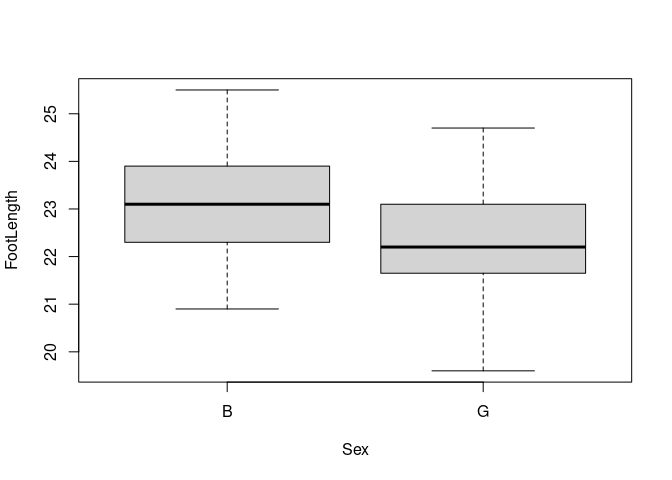
model <- lm(FootLength ~ Sex, data = feet)
summary(model)
##
## Call:
## lm(formula = FootLength ~ Sex, data = feet)
##
## Residuals:
##      Min       1Q   Median       3Q      Max
## -2.72105 -0.73684 -0.08158  0.85789  2.37895
##
## Coefficients:
##             Estimate Std. Error t value Pr(>|t|)
## (Intercept)  23.1421     0.2948  78.492   <2e-16 ***
## SexG         -0.8211     0.4170  -1.969   0.0567 .
## ---
## Signif. codes:  0 '***' 0.001 '**' 0.01 '*' 0.05 '.' 0.1 ' ' 1
##
## Residual standard error: 1.285 on 36 degrees of freedom
## Multiple R-squared:  0.09724,    Adjusted R-squared:  0.07216
## F-statistic: 3.878 on 1 and 36 DF,  p-value: 0.05667
boxplot(FootLength ~ Sex, data = feet)
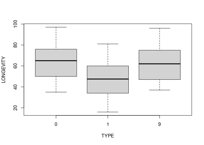
Real data: flies (A warning!)
In the slides, I covered that you need to ensure that categorical
variables are entered as such in the model. Here, is some data in which
a categorical variable is entered as a numeric variable. This is a
common mistake that can lead to incorrect results. The variable type
is a categorical variable, but it is entered as a numeric variable.
http://jse.amstat.org/datasets/fruitfly.txt
flies <- read_csv('data/flies.csv')
## Rows: 125 Columns: 6
## ── Column specification ────────────────────────────────────────────────────────
## Delimiter: ","
## dbl (6): ID, PARTNERS, TYPE, LONGEVITY, THORAX, SLEEP
##
## ℹ Use `spec()` to retrieve the full column specification for this data.
## ℹ Specify the column types or set `show_col_types = FALSE` to quiet this message.
head(flies)
## # A tibble: 6 × 6
##      ID PARTNERS  TYPE LONGEVITY THORAX SLEEP
##   <dbl>    <dbl> <dbl>     <dbl>  <dbl> <dbl>
## 1     1        8     0        35   0.64    22
## 2     2        8     0        37   0.68     9
## 3     3        8     0        49   0.68    49
## 4     4        8     0        46   0.72     1
## 5     5        8     0        63   0.72    23
## 6     6        8     0        39   0.76    83
# Don't do this!!
model <- lm(LONGEVITY ~ TYPE, data = flies)
summary(model)
##
## Call:
## lm(formula = LONGEVITY ~ TYPE, data = flies)
##
## Residuals:
##     Min      1Q  Median      3Q     Max
## -40.712 -14.105  -0.105  13.434  40.895
##
## Coefficients:
##             Estimate Std. Error t value Pr(>|t|)
## (Intercept)  56.1050     1.8607  30.152   <2e-16 ***
## TYPE          0.6068     0.4567   1.329    0.186
## ---
## Signif. codes:  0 '***' 0.001 '**' 0.01 '*' 0.05 '.' 0.1 ' ' 1
##
## Residual standard error: 17.51 on 123 degrees of freedom
## Multiple R-squared:  0.01415,    Adjusted R-squared:  0.006135
## F-statistic: 1.765 on 1 and 123 DF,  p-value: 0.1864
The ‘as.factor’ function is used to convert a numeric variable to a
categorical variable. Here, I convert the type variable to a factor
variable. Now, R will correctly encode the variable and estimate the
associated coefficients.
## Do this!!
model <- lm(LONGEVITY ~ as.factor(TYPE), data = flies)
summary(model)
##
## Call:
## lm(formula = LONGEVITY ~ as.factor(TYPE), data = flies)
##
## Residuals:
##    Min     1Q Median     3Q    Max
## -31.74 -13.74   0.26  11.44  33.26
##
## Coefficients:
##                  Estimate Std. Error t value Pr(>|t|)
## (Intercept)        64.080      2.233  28.701  < 2e-16 ***
## as.factor(TYPE)1  -16.340      3.158  -5.175 9.08e-07 ***
## as.factor(TYPE)9   -0.520      3.867  -0.134    0.893
## ---
## Signif. codes:  0 '***' 0.001 '**' 0.01 '*' 0.05 '.' 0.1 ' ' 1
##
## Residual standard error: 15.79 on 122 degrees of freedom
## Multiple R-squared:  0.2051, Adjusted R-squared:  0.1921
## F-statistic: 15.74 on 2 and 122 DF,  p-value: 8.305e-07
boxplot(LONGEVITY ~ TYPE, data = flies)
Two way ANOVA: two categorical predictors
Car noise data
Here, we will fit a linear model with two categorical predictors. The
data is from the AutoPollution dataset in the Stat2Data package. The
dataset contains information on the noise level of cars, with the
variables Size and Type encoding the size and type of the car,
respectively. Note that I convert the size and the type variables to
categorical variables.
library(Stat2Data)
data(AutoPollution)
head(AutoPollution)
##   Noise Size Type Side
## 1   810    1    1    1
## 2   820    1    1    1
## 3   820    1    1    1
## 4   840    2    1    1
## 5   840    2    1    1
## 6   845    2    1    1
AutoPollution$Size <- as.factor(AutoPollution$Size)
AutoPollution$Type <- as.factor(AutoPollution$Type)
levels(AutoPollution$Size)
## [1] "1" "2" "3"
levels(AutoPollution$Type)
## [1] "1" "2"
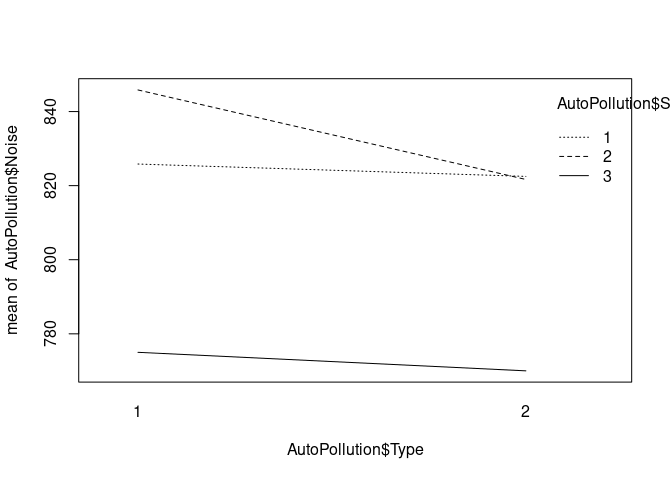
This function generates a quick plot of the data. We can compare this plot with the results of the model later.
interaction.plot(x.factor=AutoPollution$Type, trace.factor = AutoPollution$Size, response=AutoPollution$Noise)
Model without interaction
When we fit a model without interactions, its equation is the following:
\[y = \beta_0 + [\beta_1 x_1 + \beta_2 x_2 ] + [\beta_3 x_3]\]with $x_1$ and $x_2$ encoding the Variable Size and $x_3$ encoding the
variable Type.
model <- lm(Noise ~ Type + Size, data = AutoPollution)
summary(model)
##
## Call:
## lm(formula = Noise ~ Type + Size, data = AutoPollution)
##
## Residuals:
##     Min      1Q  Median      3Q     Max
## -19.583  -7.292   1.250   6.250  15.833
##
## Coefficients:
##             Estimate Std. Error t value Pr(>|t|)
## (Intercept)  829.583      3.099 267.657  < 2e-16 ***
## Type2        -10.833      3.099  -3.495  0.00141 **
## Size2          9.583      3.796   2.525  0.01674 *
## Size3        -51.667      3.796 -13.611  7.4e-15 ***
## ---
## Signif. codes:  0 '***' 0.001 '**' 0.01 '*' 0.05 '.' 0.1 ' ' 1
##
## Residual standard error: 9.298 on 32 degrees of freedom
## Multiple R-squared:  0.9074, Adjusted R-squared:  0.8987
## F-statistic: 104.5 on 3 and 32 DF,  p-value: < 2.2e-16
Model with interaction
When we fit a model with interactions, its equation is the following:
\[y = \beta_0 + [\beta_1 x_1 + \beta_2 x_2 ] + [\beta_3 x_3] + [\beta_4 x_1 x_3] + [\beta_5 x_2 x_3]\]with $x_1$ and $x_2$ encoding the Variable Size and $x_3$ encoding the
variable Type, and two terms that encode the combination of the levels
of Size and Type.
model <- lm(Noise ~ Type * Size, data = AutoPollution)
summary(model)
##
## Call:
## lm(formula = Noise ~ Type * Size, data = AutoPollution)
##
## Residuals:
##      Min       1Q   Median       3Q      Max
## -15.8333  -5.2083  -0.4167   5.0000  15.0000
##
## Coefficients:
##             Estimate Std. Error t value Pr(>|t|)
## (Intercept)  825.833      3.302 250.106  < 2e-16 ***
## Type2         -3.333      4.670  -0.714 0.480849
## Size2         20.000      4.670   4.283 0.000175 ***
## Size3        -50.833      4.670 -10.886 6.11e-12 ***
## Type2:Size2  -20.833      6.604  -3.155 0.003638 **
## Type2:Size3   -1.667      6.604  -0.252 0.802471
## ---
## Signif. codes:  0 '***' 0.001 '**' 0.01 '*' 0.05 '.' 0.1 ' ' 1
##
## Residual standard error: 8.088 on 30 degrees of freedom
## Multiple R-squared:  0.9343, Adjusted R-squared:  0.9234
## F-statistic: 85.34 on 5 and 30 DF,  p-value: < 2.2e-16
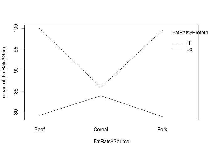
Fat rats data
data(FatRats)
head(FatRats)
##   Gain Protein Source
## 1   73      Hi   Beef
## 2  102      Hi   Beef
## 3  118      Hi   Beef
## 4  104      Hi   Beef
## 5   81      Hi   Beef
## 6  107      Hi   Beef
Protein: Level of protein (Hi or Lo)Source: Source of protein (Beef, Cereal, or Pork)
model<-lm(Gain ~ Protein * Source, data=FatRats)
summary(model)
##
## Call:
## lm(formula = Gain ~ Protein * Source, data = FatRats)
##
## Residuals:
##    Min     1Q Median     3Q    Max
##  -29.9   -8.9    2.1   10.8   27.1
##
## Coefficients:
##                        Estimate Std. Error t value Pr(>|t|)
## (Intercept)             100.000      4.628  21.607  < 2e-16 ***
## ProteinLo               -20.800      6.545  -3.178  0.00245 **
## SourceCereal            -14.100      6.545  -2.154  0.03570 *
## SourcePork               -0.500      6.545  -0.076  0.93939
## ProteinLo:SourceCereal   18.800      9.256   2.031  0.04719 *
## ProteinLo:SourcePork      0.200      9.256   0.022  0.98284
## ---
## Signif. codes:  0 '***' 0.001 '**' 0.01 '*' 0.05 '.' 0.1 ' ' 1
##
## Residual standard error: 14.64 on 54 degrees of freedom
## Multiple R-squared:  0.2835, Adjusted R-squared:  0.2172
## F-statistic: 4.273 on 5 and 54 DF,  p-value: 0.002398
interaction.plot(x.factor=FatRats$Source, trace.factor = FatRats$Protein, response= FatRats$Gain)
Change the contrasts
Here, I just quickly change the contrasts. This does not change the model’s equation (and number of fitted coefficients) but it does change the meaning of these coefficients. The sum coding compares levels to the overall mean of the response variable (the intercept is the overall mean), i.e.,
mean(FatRats$Gain)
## [1] 87.9
contrasts(FatRats$Protein) <- contr.sum(2)
contrasts(FatRats$Source) <- contr.sum(3)
model<-lm(Gain ~ Protein + Source, data=FatRats)
summary(model)
##
## Call:
## lm(formula = Gain ~ Protein + Source, data = FatRats)
##
## Residuals:
##     Min      1Q  Median      3Q     Max
## -36.133  -9.908   0.800   8.967  29.333
##
## Coefficients:
##             Estimate Std. Error t value Pr(>|t|)
## (Intercept)   87.900      1.947  45.155  < 2e-16 ***
## Protein1       7.233      1.947   3.716 0.000469 ***
## Source1        1.700      2.753   0.618 0.539399
## Source2       -3.000      2.753  -1.090 0.280500
## ---
## Signif. codes:  0 '***' 0.001 '**' 0.01 '*' 0.05 '.' 0.1 ' ' 1
##
## Residual standard error: 15.08 on 56 degrees of freedom
## Multiple R-squared:  0.2113, Adjusted R-squared:  0.169
## F-statistic: 5.001 on 3 and 56 DF,  p-value: 0.003834
Interpreting the coefficients
The sum contrast compares each level of a variable to the overall mean. It is important to remember that knowing a variable’s mean value and n deviations from this mean allows us to fix n + 1 values. This mechanism is used by deviation coding to model the various levels of the dependent given the independent.
The overall mean for the dependent is 87.9. The fitted coefficient for
Protein is 7.233. This means that for one level of this variable the
average should be (87.9 + 7.233) = 95.133. For the other level, the
average should be 87.9 - 7.233) = 80.667. Indeed, if this were not so,
the overall mean could not be 87.9.
We can see that is so by calculating the average of the dependent
variable for the two levels of Protein:
grouped <- group_by(FatRats, Protein)
means <- summarise(grouped, mean = mean(Gain))
means
## # A tibble: 2 × 2
##   Protein  mean
##   <fct>   <dbl>
## 1 Hi       95.1
## 2 Lo       80.7
For the variable Source a similar reasoning holds.
For one level of the variable, the average dependent should be (87.9 +1.7) = 89.6. For another, the average should be (87.9 -3) = 84.9. Finally, to ensure that the average is 87.9, the last level should have a mean of 87.9 - (1.7 + -3) = 89.2.
grouped <- group_by(FatRats, Source)
means <- summarise(grouped, mean = mean(Gain))
means
## # A tibble: 3 × 2
##   Source  mean
##   <fct>  <dbl>
## 1 Beef    89.6
## 2 Cereal  84.9
## 3 Pork    89.2