Multiple Regression
Dieter Last Updated: 04, December, 2025 at 09:20
- Data used
- Read in some data
- Revisit the simple linear model
- Intro to the multiple linear regression
- Model comparison
- Interactions
- Step
Data used
body.csvvik_table_9_2.csv
Read in some data
library(tidyverse)
## ── Attaching core tidyverse packages ──────────────────────── tidyverse 2.0.0 ──
## ✔ dplyr     1.1.4     ✔ readr     2.1.5
## ✔ forcats   1.0.1     ✔ stringr   1.5.2
## ✔ ggplot2   4.0.0     ✔ tibble    3.3.0
## ✔ lubridate 1.9.4     ✔ tidyr     1.3.1
## ✔ purrr     1.1.0
## ── Conflicts ────────────────────────────────────────── tidyverse_conflicts() ──
## ✖ dplyr::filter() masks stats::filter()
## ✖ dplyr::lag()    masks stats::lag()
## ℹ Use the conflicted package (<http://conflicted.r-lib.org/>) to force all conflicts to become errors
body_data <-read_csv('data/body.csv')
## Rows: 507 Columns: 25
## ── Column specification ────────────────────────────────────────────────────────
## Delimiter: ","
## dbl (25): Biacromial, Biiliac, Bitrochanteric, ChestDepth, ChestDia, ElbowDi...
##
## ℹ Use `spec()` to retrieve the full column specification for this data.
## ℹ Specify the column types or set `show_col_types = FALSE` to quiet this message.
Revisit the simple linear model
This is a quick recap of the simple linear regression model.
model <- lm(Weight ~ Waist, data=body_data)
summary(model)
##
## Call:
## lm(formula = Weight ~ Waist, data = body_data)
##
## Residuals:
##      Min       1Q   Median       3Q      Max
## -16.3211  -3.5995  -0.0936   3.6932  19.0536
##
## Coefficients:
##              Estimate Std. Error t value Pr(>|t|)
## (Intercept) -15.18382    1.79291  -8.469 2.72e-16 ***
## Waist         1.09550    0.02306  47.514  < 2e-16 ***
## ---
## Signif. codes:  0 '***' 0.001 '**' 0.01 '*' 0.05 '.' 0.1 ' ' 1
##
## Residual standard error: 5.712 on 505 degrees of freedom
## Multiple R-squared:  0.8172, Adjusted R-squared:  0.8168
## F-statistic:  2258 on 1 and 505 DF,  p-value: < 2.2e-16
The anova table shows more details about the components calculating the F-value
anova(model)
## Analysis of Variance Table
##
## Response: Weight
##            Df Sum Sq Mean Sq F value    Pr(>F)
## Waist       1  73649   73649  2257.6 < 2.2e-16 ***
## Residuals 505  16475      33
## ---
## Signif. codes:  0 '***' 0.001 '**' 0.01 '*' 0.05 '.' 0.1 ' ' 1
Manual calculation of the F value
As we mentioned before, R automatically calculates the F-value. But we can also do this manually. You an inspect this code if you want to understand the calculation of the F value in more detail.
predicted <- predict(model)
mn_predicted <-mean(predicted)
resids <- model$residuals


captured_variance <- sum((predicted - mn_predicted)^2)
uncaptured_variance <- sum((resids)^2)

n_predictors <- 1
manual_f <- (captured_variance / n_predictors)/ (uncaptured_variance/ model$df.residual)
captured_variance
## [1] 73648.74
uncaptured_variance
## [1] 16474.61
manual_f
## [1] 2257.572
Intro to the multiple linear regression
A first example
Here I use data provided by Vik 2013 (Table 9.2 in Vik, Peter. Regression, ANOVA, and the General Linear Model, 2013.). This allows double checking the calculations provided in this book.
vik_data <-read_csv('data/vik_table_9_2.csv')
## Rows: 12 Columns: 4
## ── Column specification ────────────────────────────────────────────────────────
## Delimiter: ","
## dbl (4): Person, Y, X1, X2
##
## ℹ Use `spec()` to retrieve the full column specification for this data.
## ℹ Specify the column types or set `show_col_types = FALSE` to quiet this message.
head(vik_data)
## # A tibble: 6 × 4
##   Person     Y    X1    X2
##    <dbl> <dbl> <dbl> <dbl>
## 1      1     2     8     1
## 2      2     3     9     2
## 3      3     3     9     2
## 4      4     4    10     3
## 5      5     7     6     8
## 6      6     5     7     9
model <- lm(Y ~ X1 + X2, data=vik_data)
summary(model)
##
## Call:
## lm(formula = Y ~ X1 + X2, data = vik_data)
##
## Residuals:
##      Min       1Q   Median       3Q      Max
## -2.45564 -0.24631  0.03248  0.54747  1.52060
##
## Coefficients:
##             Estimate Std. Error t value Pr(>|t|)
## (Intercept)   9.2014     1.5185   6.060 0.000188 ***
## X1           -0.7085     0.1481  -4.783 0.000997 ***
## X2            0.1209     0.1486   0.813 0.436963
## ---
## Signif. codes:  0 '***' 0.001 '**' 0.01 '*' 0.05 '.' 0.1 ' ' 1
##
## Residual standard error: 1.271 on 9 degrees of freedom
## Multiple R-squared:  0.8182, Adjusted R-squared:  0.7777
## F-statistic: 20.25 on 2 and 9 DF,  p-value: 0.0004663
Manual calculation of the F value
Just as before, we can calculate the F value manually to get a better understanding of the calculation of F.
predicted <- predict(model)
mn_predicted <-mean(predicted)
resids <- model$residuals

captured_variance <- sum((predicted - mn_predicted)^2)
uncaptured_variance <- sum((resids)^2)

n_predictors <- 2
manual_F <- (captured_variance / n_predictors)/ (uncaptured_variance/ model$df.residual)
captured_variance
## [1] 65.45267
uncaptured_variance
## [1] 14.54733
manual_f
## [1] 2257.572
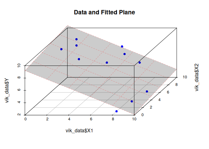
Visualizing the fitted model
library(scatterplot3d)

# Fit model
model <- lm(Y ~ X1 + X2, data = vik_data)

# Create grid for the plane
xg <- seq(min(vik_data$X1), max(vik_data$X1), length.out = 20)
yg <- seq(min(vik_data$X2), max(vik_data$X2), length.out = 20)
grid <- expand.grid(X1 = xg, X2 = yg)

grid$Z <- predict(model, newdata = grid)

# Draw scatter
s3d <- scatterplot3d(
  x = vik_data$X1,
  y = vik_data$X2,
  z = vik_data$Y,
  pch = 16,
  color = "blue",
  angle = 55,
  main = "Data and Fitted Plane"
)

# Add plane
s3d$plane3d(model, draw_polygon = TRUE, col = rgb(1, 0, 0, 0.3))
Manually running the omnibus test
I fit the full model and the base model (which is usually only done implicitly). We fit the following two models:
\[y_i = \bar{y}\] \[y_i = \beta_0 + \beta_1 x_{1i} + \beta_2 x_{2i}\]Next, we explicitly compare their performances using the anova
function. This results in the same F-value as the one calculated by R
when fitting the full model.
vik_data$mean_y <- mean(vik_data$Y)


model_base <- lm(Y ~ mean_y, data=vik_data)
model_full <- lm(Y ~ X1 + X2, data=vik_data)
Let’s look at the full model’s F value.
summary(model_full)
##
## Call:
## lm(formula = Y ~ X1 + X2, data = vik_data)
##
## Residuals:
##      Min       1Q   Median       3Q      Max
## -2.45564 -0.24631  0.03248  0.54747  1.52060
##
## Coefficients:
##             Estimate Std. Error t value Pr(>|t|)
## (Intercept)   9.2014     1.5185   6.060 0.000188 ***
## X1           -0.7085     0.1481  -4.783 0.000997 ***
## X2            0.1209     0.1486   0.813 0.436963
## ---
## Signif. codes:  0 '***' 0.001 '**' 0.01 '*' 0.05 '.' 0.1 ' ' 1
##
## Residual standard error: 1.271 on 9 degrees of freedom
## Multiple R-squared:  0.8182, Adjusted R-squared:  0.7777
## F-statistic: 20.25 on 2 and 9 DF,  p-value: 0.0004663
Let’s now explicitly compare the base and the full model. This results in the same F-value! So, we could run the omnibus test by comparing the base model, $y_i = \bar{x}$, with the full model. But this is done implicitly by R when fitting the full model.
anova(model_base, model_full)
## Analysis of Variance Table
##
## Model 1: Y ~ mean_y
## Model 2: Y ~ X1 + X2
##   Res.Df    RSS Df Sum of Sq      F    Pr(>F)
## 1     11 80.000
## 2      9 14.547  2    65.453 20.247 0.0004663 ***
## ---
## Signif. codes:  0 '***' 0.001 '**' 0.01 '*' 0.05 '.' 0.1 ' ' 1
Manually calculating the F ratio for the omnibus test
full_model_predictions <- predict(model_full)
mean_full_model_predictions <-mean(full_model_predictions)

base_model_predictions <- predict(model_base)

captured_variance <- sum((full_model_predictions - mean_full_model_predictions)^2)
uncaptured_variance <- sum((base_model_predictions- vik_data$Y)^2)
test <- sum((model_full$residuals)^2)
test
## [1] 14.54733
captured_variance
## [1] 65.45267
uncaptured_variance
## [1] 80
manual_f <- captured_variance/uncaptured_variance
manual_f
## [1] 0.8181584
Model comparison
Here, we fit two nested models and compare their performance using the
anova function. The simple model uses only Illiteracy to predict a
state’s Murder rate, while the complex model adds two additional
predictors: Income and Population.
Because the simple model is nested within the complex one, we can
formally evaluate whether the extra variables provide a meaningful
improvement in explanatory power. After examining the model summaries,
we use the anova() function to compare the two fits. This test
quantifies whether the reduction in residual error achieved by the more
complex model is large enough to justify its additional parameters.
A simple and a complex model
state_data <- as.data.frame(state.x77)
colnames(state_data) <- make.names(colnames(state_data))
head(state_data)
##            Population Income Illiteracy Life.Exp Murder HS.Grad Frost   Area
## Alabama          3615   3624        2.1    69.05   15.1    41.3    20  50708
## Alaska            365   6315        1.5    69.31   11.3    66.7   152 566432
## Arizona          2212   4530        1.8    70.55    7.8    58.1    15 113417
## Arkansas         2110   3378        1.9    70.66   10.1    39.9    65  51945
## California      21198   5114        1.1    71.71   10.3    62.6    20 156361
## Colorado         2541   4884        0.7    72.06    6.8    63.9   166 103766
Let’s fit two (nested) models,
simple_model <- lm(state_data$Murder ~ state_data$Illiteracy)
complex_model <- lm(state_data$Murder ~ state_data$Illiteracy + state_data$Income + state_data$Population)
Let’s look at their summaries:
summary(simple_model)
##
## Call:
## lm(formula = state_data$Murder ~ state_data$Illiteracy)
##
## Residuals:
##     Min      1Q  Median      3Q     Max
## -5.5315 -2.0602 -0.2503  1.6916  6.9745
##
## Coefficients:
##                       Estimate Std. Error t value Pr(>|t|)
## (Intercept)             2.3968     0.8184   2.928   0.0052 **
## state_data$Illiteracy   4.2575     0.6217   6.848 1.26e-08 ***
## ---
## Signif. codes:  0 '***' 0.001 '**' 0.01 '*' 0.05 '.' 0.1 ' ' 1
##
## Residual standard error: 2.653 on 48 degrees of freedom
## Multiple R-squared:  0.4942, Adjusted R-squared:  0.4836
## F-statistic: 46.89 on 1 and 48 DF,  p-value: 1.258e-08
summary(complex_model)
##
## Call:
## lm(formula = state_data$Murder ~ state_data$Illiteracy + state_data$Income +
##     state_data$Population)
##
## Residuals:
##     Min      1Q  Median      3Q     Max
## -4.7846 -1.6768 -0.0839  1.4783  7.6417
##
## Coefficients:
##                        Estimate Std. Error t value Pr(>|t|)
## (Intercept)           1.3402721  3.3694210   0.398   0.6926
## state_data$Illiteracy 4.1109188  0.6706786   6.129 1.85e-07 ***
## state_data$Income     0.0000644  0.0006762   0.095   0.9245
## state_data$Population 0.0002219  0.0000842   2.635   0.0114 *
## ---
## Signif. codes:  0 '***' 0.001 '**' 0.01 '*' 0.05 '.' 0.1 ' ' 1
##
## Residual standard error: 2.507 on 46 degrees of freedom
## Multiple R-squared:  0.5669, Adjusted R-squared:  0.5387
## F-statistic: 20.07 on 3 and 46 DF,  p-value: 1.84e-08
anova(simple_model, complex_model)
## Analysis of Variance Table
##
## Model 1: state_data$Murder ~ state_data$Illiteracy
## Model 2: state_data$Murder ~ state_data$Illiteracy + state_data$Income +
##     state_data$Population
##   Res.Df    RSS Df Sum of Sq      F  Pr(>F)
## 1     48 337.76
## 2     46 289.19  2    48.574 3.8633 0.02812 *
## ---
## Signif. codes:  0 '***' 0.001 '**' 0.01 '*' 0.05 '.' 0.1 ' ' 1
What if the models only differ by one variable
When two models differ by only one additional predictor, the hypothesis
test reported in the model summary and the test produced by anova()
are mathematically and logically equivalent.
The p-value for the new variable in the regression output tests whether its coefficient differs significantly from zero, and the ANOVA comparison tests whether adding that variable produces a meaningful reduction in residual error. Because both procedures evaluate the same hypothesis, their test statistics are directly related: the p-value associated with the newly introduced variable is equal to the $p$ value of the anova comparison. In fact the $F$ value is equal to $t^2$ value.
simple_model <- lm(state_data$Murder ~ state_data$Illiteracy)
complex_model <- lm(state_data$Murder ~ state_data$Illiteracy + state_data$Income)
summary(complex_model)
##
## Call:
## lm(formula = state_data$Murder ~ state_data$Illiteracy + state_data$Income)
##
## Residuals:
##     Min      1Q  Median      3Q     Max
## -5.6343 -1.9289 -0.0171  1.6779  6.7349
##
## Coefficients:
##                         Estimate Std. Error t value Pr(>|t|)
## (Intercept)           -0.4409926  3.5034602  -0.126    0.900
## state_data$Illiteracy  4.5099882  0.6934465   6.504 4.63e-08 ***
## state_data$Income      0.0005731  0.0006879   0.833    0.409
## ---
## Signif. codes:  0 '***' 0.001 '**' 0.01 '*' 0.05 '.' 0.1 ' ' 1
##
## Residual standard error: 2.661 on 47 degrees of freedom
## Multiple R-squared:  0.5015, Adjusted R-squared:  0.4803
## F-statistic: 23.64 on 2 and 47 DF,  p-value: 7.841e-08
anova(simple_model, complex_model)
## Analysis of Variance Table
##
## Model 1: state_data$Murder ~ state_data$Illiteracy
## Model 2: state_data$Murder ~ state_data$Illiteracy + state_data$Income
##   Res.Df    RSS Df Sum of Sq      F Pr(>F)
## 1     48 337.76
## 2     47 332.85  1    4.9163 0.6942 0.4089
Interactions
Model without interaction
library(gapminder)
gap <- gapminder
model <- lm(lifeExp ~ gdpPercap + year, data = gap)
summary(model)
##
## Call:
## lm(formula = lifeExp ~ gdpPercap + year, data = gap)
##
## Residuals:
##     Min      1Q  Median      3Q     Max
## -67.262  -6.954   1.219   7.759  19.553
##
## Coefficients:
##               Estimate Std. Error t value Pr(>|t|)
## (Intercept) -4.184e+02  2.762e+01  -15.15   <2e-16 ***
## gdpPercap    6.697e-04  2.447e-05   27.37   <2e-16 ***
## year         2.390e-01  1.397e-02   17.11   <2e-16 ***
## ---
## Signif. codes:  0 '***' 0.001 '**' 0.01 '*' 0.05 '.' 0.1 ' ' 1
##
## Residual standard error: 9.694 on 1701 degrees of freedom
## Multiple R-squared:  0.4375, Adjusted R-squared:  0.4368
## F-statistic: 661.4 on 2 and 1701 DF,  p-value: < 2.2e-16
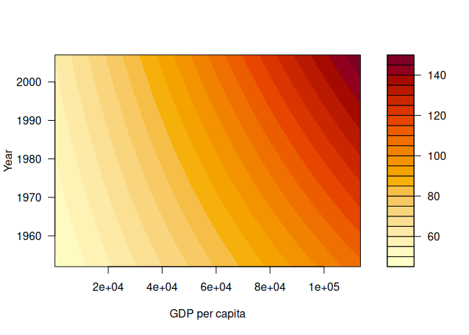
Model with interaction
An interaction term allows the regression model to capture situations where the effect of one predictor is not constant but depends on the level of another predictor. In this example, including the product GDP × YEAR means that the relationship between GDP per capita and life expectancy can change over time.
model <- lm(lifeExp ~ gdpPercap * year, data = gap)
summary(model)
##
## Call:
## lm(formula = lifeExp ~ gdpPercap * year, data = gap)
##
## Residuals:
##     Min      1Q  Median      3Q     Max
## -54.234  -7.314   1.002   7.951  19.780
##
## Coefficients:
##                  Estimate Std. Error t value Pr(>|t|)
## (Intercept)    -3.532e+02  3.267e+01 -10.811  < 2e-16 ***
## gdpPercap      -8.754e-03  2.547e-03  -3.437 0.000602 ***
## year            2.060e-01  1.653e-02  12.463  < 2e-16 ***
## gdpPercap:year  4.754e-06  1.285e-06   3.700 0.000222 ***
## ---
## Signif. codes:  0 '***' 0.001 '**' 0.01 '*' 0.05 '.' 0.1 ' ' 1
##
## Residual standard error: 9.658 on 1700 degrees of freedom
## Multiple R-squared:  0.442,  Adjusted R-squared:  0.441
## F-statistic: 448.8 on 3 and 1700 DF,  p-value: < 2.2e-16
This fits the following model:
\[L = \beta_0 + \beta_1 \text{GDP} + \beta_2 \text{YEAR} + \beta_3 \text{GDP} \times \text{YEAR}\]As shown in the slides, this mathematically equivalent to:
\[L = \beta_0 + \beta_1 \text{GDP} + [\beta_2 + \beta_3 \text{GDP}] \times \text{YEAR}\]or
\(L = \beta_0 + \beta_1 \text{YEAR} + [\beta_1 + \beta_3 \text{YEAR}] \times \text{GDP}\) This can be interpreted as stating that the effect of GPD is modified by year. Or that the effect of year is modified by GPD.
The code below shows the fitted surface.
x_range <- seq(241, 113523, length.out = 200)   # GDP per capita
y_range <- seq(1952, 2007, length.out = 200)    # Year
grid <- expand.grid(gdpPercap = x_range, year = y_range)
grid$lifeExp_pred <- predict(model, newdata = grid)
z_matrix <- matrix(grid$lifeExp_pred, nrow = length(x_range), ncol = length(y_range))

filled.contour(x = x_range, y = y_range, z = z_matrix, xlab = "GDP per capita", ylab = "Year")
I also plotted the model in the wolfram alpha. See this link for a plot of the model: https://www.wolframalpha.com/input?i=plot+-3.532e%2B02+%2B+x+*+-8.754e-03+%2B+y+*+2.060e-01+%2B+4.754e-06+*+%28x+*+y%29+with+x++%3D+241+to+113523+and+y+%3D+1952+to+2007
This gives the same result:
gap$multi <- gap$gdpPercap * gap$year
model <- lm(lifeExp ~ gdpPercap + year + multi, data = gap)
summary(model)
##
## Call:
## lm(formula = lifeExp ~ gdpPercap + year + multi, data = gap)
##
## Residuals:
##     Min      1Q  Median      3Q     Max
## -54.234  -7.314   1.002   7.951  19.780
##
## Coefficients:
##               Estimate Std. Error t value Pr(>|t|)
## (Intercept) -3.532e+02  3.267e+01 -10.811  < 2e-16 ***
## gdpPercap   -8.754e-03  2.547e-03  -3.437 0.000602 ***
## year         2.060e-01  1.653e-02  12.463  < 2e-16 ***
## multi        4.754e-06  1.285e-06   3.700 0.000222 ***
## ---
## Signif. codes:  0 '***' 0.001 '**' 0.01 '*' 0.05 '.' 0.1 ' ' 1
##
## Residual standard error: 9.658 on 1700 degrees of freedom
## Multiple R-squared:  0.442,  Adjusted R-squared:  0.441
## F-statistic: 448.8 on 3 and 1700 DF,  p-value: < 2.2e-16
Using zeroed data
We now standardize YEAR and GDP so that 0 means ‘average year’ and ‘average GDP’. This makes the interaction coefficients easier to interpret. It also reduces collinearity between the main effects and the interaction term.
gap <- mutate(gap, year = scale(year))
gap <- mutate(gap, gdpPercap = scale(gdpPercap))
model <- lm(lifeExp ~ gdpPercap * year, data = gap)
range(gap$gdpPercap)
## [1] -0.7075012 10.7845089
range(gap$year)
## [1] -1.592787 1.592787
summary(model)
##
## Call:
## lm(formula = lifeExp ~ gdpPercap * year, data = gap)
##
## Residuals:
##     Min      1Q  Median      3Q     Max
## -54.234  -7.314   1.002   7.951  19.780
##
## Coefficients:
##                Estimate Std. Error t value Pr(>|t|)
## (Intercept)     59.2906     0.2392  247.90  < 2e-16 ***
## gdpPercap        6.4680     0.2430   26.61  < 2e-16 ***
## year             4.1489     0.2404   17.26  < 2e-16 ***
## gdpPercap:year   0.8091     0.2187    3.70 0.000222 ***
## ---
## Signif. codes:  0 '***' 0.001 '**' 0.01 '*' 0.05 '.' 0.1 ' ' 1
##
## Residual standard error: 9.658 on 1700 degrees of freedom
## Multiple R-squared:  0.442,  Adjusted R-squared:  0.441
## F-statistic: 448.8 on 3 and 1700 DF,  p-value: < 2.2e-16
The fitted model becomes,
\(z = 59.29 + 6.46 x + 4.14 y + 0.80 + x y\) with $x$ the gdpPercap and $y$ the year.
See this link for a graph: https://www.wolframalpha.com/input?i=plot+59.2906+%2B+6.4680+*+x+%2B+4.1489+*+y+%2B+0.8091+%2B+x+*+y+with+x+from+-+1+to+11+and+y+from+-2+to+2
Step
Using the Murder data
library(MASS)
##
## Attaching package: 'MASS'

## The following object is masked from 'package:dplyr':
##
##     select
full=lm(Murder~.,data=state_data)
stepAIC(full, direction="backward", trace = TRUE)
## Start:  AIC=63.01
## Murder ~ Population + Income + Illiteracy + Life.Exp + HS.Grad +
##     Frost + Area
##
##              Df Sum of Sq    RSS    AIC
## - Income      1     0.236 128.27 61.105
## - HS.Grad     1     0.973 129.01 61.392
## <none>                    128.03 63.013
## - Area        1     7.514 135.55 63.865
## - Illiteracy  1     8.299 136.33 64.154
## - Frost       1     9.260 137.29 64.505
## - Population  1    25.719 153.75 70.166
## - Life.Exp    1   127.175 255.21 95.503
##
## Step:  AIC=61.11
## Murder ~ Population + Illiteracy + Life.Exp + HS.Grad + Frost +
##     Area
##
##              Df Sum of Sq    RSS    AIC
## - HS.Grad     1     0.763 129.03 59.402
## <none>                    128.27 61.105
## - Area        1     7.310 135.58 61.877
## - Illiteracy  1     8.715 136.98 62.392
## - Frost       1     9.345 137.61 62.621
## - Population  1    27.142 155.41 68.702
## - Life.Exp    1   127.500 255.77 93.613
##
## Step:  AIC=59.4
## Murder ~ Population + Illiteracy + Life.Exp + Frost + Area
##
##              Df Sum of Sq    RSS    AIC
## <none>                    129.03 59.402
## - Illiteracy  1     8.723 137.75 60.672
## - Frost       1    11.030 140.06 61.503
## - Area        1    15.937 144.97 63.225
## - Population  1    26.415 155.45 66.714
## - Life.Exp    1   140.391 269.42 94.213

##
## Call:
## lm(formula = Murder ~ Population + Illiteracy + Life.Exp + Frost +
##     Area, data = state_data)
##
## Coefficients:
## (Intercept)   Population   Illiteracy     Life.Exp        Frost         Area
##   1.202e+02    1.780e-04    1.173e+00   -1.608e+00   -1.373e-02    6.804e-06
Using the body data
library(MASS)
full=lm(Weight~.,data=body_data)
stepAIC(full, direction="backward", trace = TRUE)
## Start:  AIC=775.52
## Weight ~ Biacromial + Biiliac + Bitrochanteric + ChestDepth +
##     ChestDia + ElbowDia + WristDia + KneeDia + AnkleDia + Shoulder +
##     Chest + Waist + Navel + Hip + Thigh + Bicep + Forearm + Knee +
##     Calf + Ankle + Wrist + Age + Height + Gender
##
##                  Df Sum of Sq    RSS    AIC
## - Ankle           1      0.06 2120.8 773.54
## - Navel           1      0.49 2121.2 773.64
## - Biacromial      1      0.71 2121.5 773.69
## - AnkleDia        1      2.08 2122.8 774.02
## - WristDia        1      3.42 2124.2 774.34
## - Bitrochanteric  1      3.83 2124.6 774.44
## - Wrist           1      5.98 2126.7 774.95
## - ElbowDia        1      6.57 2127.3 775.09
## - Bicep           1      8.17 2128.9 775.47
## <none>                        2120.7 775.52
## - Biiliac         1     13.13 2133.9 776.65
## - ChestDia        1     15.71 2136.5 777.27
## - Shoulder        1     27.81 2148.6 780.13
## - Knee            1     30.39 2151.1 780.74
## - Gender          1     36.02 2156.8 782.06
## - KneeDia         1     43.48 2164.2 783.81
## - Chest           1     47.62 2168.4 784.78
## - Forearm         1     51.49 2172.2 785.69
## - ChestDepth      1     77.87 2198.6 791.81
## - Thigh           1     78.65 2199.4 791.99
## - Age             1     88.97 2209.7 794.36
## - Hip             1    108.21 2229.0 798.75
## - Calf            1    118.89 2239.6 801.18
## - Waist           1    797.97 2918.7 935.45
## - Height          1   1173.76 3294.5 996.85
##
## Step:  AIC=773.54
## Weight ~ Biacromial + Biiliac + Bitrochanteric + ChestDepth +
##     ChestDia + ElbowDia + WristDia + KneeDia + AnkleDia + Shoulder +
##     Chest + Waist + Navel + Hip + Thigh + Bicep + Forearm + Knee +
##     Calf + Wrist + Age + Height + Gender
##
##                  Df Sum of Sq    RSS    AIC
## - Navel           1      0.46 2121.3 771.65
## - Biacromial      1      0.69 2121.5 771.70
## - AnkleDia        1      2.46 2123.3 772.13
## - WristDia        1      3.37 2124.2 772.34
## - Bitrochanteric  1      3.80 2124.6 772.45
## - Wrist           1      6.08 2126.9 772.99
## - ElbowDia        1      6.52 2127.3 773.09
## - Bicep           1      8.15 2129.0 773.48
## <none>                        2120.8 773.54
## - Biiliac         1     13.10 2133.9 774.66
## - ChestDia        1     15.71 2136.5 775.28
## - Shoulder        1     27.86 2148.7 778.15
## - Knee            1     32.75 2153.6 779.31
## - Gender          1     36.02 2156.8 780.08
## - KneeDia         1     43.87 2164.7 781.92
## - Chest           1     47.59 2168.4 782.79
## - Forearm         1     51.43 2172.2 783.69
## - ChestDepth      1     77.84 2198.6 789.81
## - Thigh           1     78.76 2199.6 790.02
## - Age             1     89.71 2210.5 792.54
## - Hip             1    108.59 2229.4 796.86
## - Calf            1    137.71 2258.5 803.44
## - Waist           1    798.17 2919.0 933.49
## - Height          1   1174.23 3295.0 994.93
##
## Step:  AIC=771.65
## Weight ~ Biacromial + Biiliac + Bitrochanteric + ChestDepth +
##     ChestDia + ElbowDia + WristDia + KneeDia + AnkleDia + Shoulder +
##     Chest + Waist + Hip + Thigh + Bicep + Forearm + Knee + Calf +
##     Wrist + Age + Height + Gender
##
##                  Df Sum of Sq    RSS    AIC
## - Biacromial      1      0.66 2121.9 769.81
## - AnkleDia        1      2.22 2123.5 770.18
## - Bitrochanteric  1      3.57 2124.8 770.50
## - WristDia        1      3.64 2124.9 770.52
## - Wrist           1      6.05 2127.3 771.09
## - ElbowDia        1      6.26 2127.5 771.14
## - Bicep           1      7.75 2129.0 771.50
## <none>                        2121.3 771.65
## - Biiliac         1     12.67 2133.9 772.67
## - ChestDia        1     16.22 2137.5 773.51
## - Shoulder        1     28.62 2149.9 776.44
## - Knee            1     32.29 2153.6 777.31
## - Gender          1     36.57 2157.8 778.31
## - KneeDia         1     45.28 2166.6 780.36
## - Chest           1     47.13 2168.4 780.79
## - Forearm         1     52.51 2173.8 782.05
## - ChestDepth      1     77.39 2198.7 787.82
## - Thigh           1     81.25 2202.5 788.71
## - Age             1     96.82 2218.1 792.28
## - Hip             1    121.11 2242.4 797.80
## - Calf            1    140.97 2262.2 802.27
## - Waist           1    896.91 3018.2 948.44
## - Height          1   1174.61 3295.9 993.06
##
## Step:  AIC=769.81
## Weight ~ Biiliac + Bitrochanteric + ChestDepth + ChestDia + ElbowDia +
##     WristDia + KneeDia + AnkleDia + Shoulder + Chest + Waist +
##     Hip + Thigh + Bicep + Forearm + Knee + Calf + Wrist + Age +
##     Height + Gender
##
##                  Df Sum of Sq    RSS    AIC
## - AnkleDia        1      2.48 2124.4 768.40
## - WristDia        1      3.67 2125.6 768.68
## - Bitrochanteric  1      4.29 2126.2 768.83
## - ElbowDia        1      6.13 2128.1 769.27
## - Wrist           1      6.92 2128.9 769.46
## - Bicep           1      8.26 2130.2 769.78
## <none>                        2121.9 769.81
## - Biiliac         1     12.23 2134.2 770.72
## - ChestDia        1     15.56 2137.5 771.51
## - Shoulder        1     28.16 2150.1 774.49
## - Knee            1     32.95 2154.9 775.62
## - Gender          1     40.48 2162.4 777.39
## - KneeDia         1     44.74 2166.7 778.39
## - Chest           1     48.22 2170.2 779.20
## - Forearm         1     52.71 2174.6 780.25
## - ChestDepth      1     77.31 2199.2 785.95
## - Thigh           1     81.31 2203.2 786.87
## - Age             1     96.41 2218.3 790.33
## - Hip             1    123.57 2245.5 796.50
## - Calf            1    140.68 2262.6 800.35
## - Waist           1    897.14 3019.1 946.59
## - Height          1   1219.78 3341.7 998.06
##
## Step:  AIC=768.4
## Weight ~ Biiliac + Bitrochanteric + ChestDepth + ChestDia + ElbowDia +
##     WristDia + KneeDia + Shoulder + Chest + Waist + Hip + Thigh +
##     Bicep + Forearm + Knee + Calf + Wrist + Age + Height + Gender
##
##                  Df Sum of Sq    RSS     AIC
## - Bitrochanteric  1      4.47 2128.9  767.46
## - WristDia        1      4.54 2129.0  767.48
## - Wrist           1      6.39 2130.8  767.92
## - Bicep           1      7.91 2132.3  768.28
## <none>                        2124.4  768.40
## - ElbowDia        1      9.46 2133.9  768.65
## - Biiliac         1     13.47 2137.9  769.60
## - ChestDia        1     15.43 2139.8  770.07
## - Shoulder        1     26.32 2150.7  772.64
## - Knee            1     31.67 2156.1  773.90
## - Gender          1     38.79 2163.2  775.57
## - Chest           1     51.66 2176.1  778.58
## - Forearm         1     51.96 2176.4  778.65
## - KneeDia         1     53.53 2177.9  779.02
## - ChestDepth      1     77.05 2201.5  784.46
## - Thigh           1     82.29 2206.7  785.67
## - Age             1     94.35 2218.8  788.43
## - Hip             1    122.97 2247.4  794.93
## - Calf            1    143.48 2267.9  799.53
## - Waist           1    896.31 3020.7  944.86
## - Height          1   1255.96 3380.4 1001.90
##
## Step:  AIC=767.46
## Weight ~ Biiliac + ChestDepth + ChestDia + ElbowDia + WristDia +
##     KneeDia + Shoulder + Chest + Waist + Hip + Thigh + Bicep +
##     Forearm + Knee + Calf + Wrist + Age + Height + Gender
##
##              Df Sum of Sq    RSS     AIC
## - WristDia    1      4.90 2133.8  766.63
## - Wrist       1      6.96 2135.8  767.12
## - Bicep       1      7.34 2136.2  767.21
## - ElbowDia    1      7.67 2136.6  767.29
## <none>                    2128.9  767.46
## - Biiliac     1      9.65 2138.5  767.76
## - ChestDia    1     12.91 2141.8  768.53
## - Shoulder    1     27.13 2156.0  771.88
## - Knee        1     33.25 2162.1  773.32
## - Gender      1     39.54 2168.4  774.79
## - KneeDia     1     51.57 2180.5  777.60
## - Forearm     1     54.44 2183.3  778.27
## - Chest       1     57.69 2186.6  779.02
## - ChestDepth  1     77.06 2205.9  783.49
## - Thigh       1     87.77 2216.7  785.95
## - Age         1     99.38 2228.3  788.60
## - Hip         1    127.01 2255.9  794.84
## - Calf        1    139.66 2268.5  797.68
## - Waist       1    911.72 3040.6  946.19
## - Height      1   1254.46 3383.3 1000.34
##
## Step:  AIC=766.63
## Weight ~ Biiliac + ChestDepth + ChestDia + ElbowDia + KneeDia +
##     Shoulder + Chest + Waist + Hip + Thigh + Bicep + Forearm +
##     Knee + Calf + Wrist + Age + Height + Gender
##
##              Df Sum of Sq    RSS     AIC
## - Wrist       1      3.97 2137.7  765.57
## - Bicep       1      7.13 2140.9  766.32
## <none>                    2133.8  766.63
## - Biiliac     1      9.23 2143.0  766.82
## - ElbowDia    1     12.10 2145.9  767.49
## - ChestDia    1     13.55 2147.3  767.84
## - Shoulder    1     26.56 2160.3  770.90
## - Knee        1     32.84 2166.6  772.37
## - Gender      1     39.48 2173.3  773.92
## - Forearm     1     54.13 2187.9  777.33
## - KneeDia     1     56.85 2190.6  777.96
## - Chest       1     60.08 2193.9  778.71
## - ChestDepth  1     73.88 2207.7  781.89
## - Thigh       1     85.73 2219.5  784.60
## - Age         1     97.74 2231.5  787.34
## - Hip         1    127.75 2261.5  794.11
## - Calf        1    142.03 2275.8  797.30
## - Waist       1    917.62 3051.4  945.99
## - Height      1   1271.05 3404.8 1001.55
##
## Step:  AIC=765.57
## Weight ~ Biiliac + ChestDepth + ChestDia + ElbowDia + KneeDia +
##     Shoulder + Chest + Waist + Hip + Thigh + Bicep + Forearm +
##     Knee + Calf + Age + Height + Gender
##
##              Df Sum of Sq    RSS     AIC
## - Bicep       1      6.68 2144.4  765.15
## <none>                    2137.7  765.57
## - ElbowDia    1     11.05 2148.8  766.18
## - Biiliac     1     11.41 2149.2  766.27
## - ChestDia    1     14.04 2151.8  766.89
## - Shoulder    1     26.62 2164.4  769.85
## - Knee        1     31.10 2168.8  770.89
## - Gender      1     39.75 2177.5  772.91
## - Forearm     1     50.51 2188.3  775.41
## - KneeDia     1     53.43 2191.2  776.09
## - Chest       1     58.40 2196.1  777.24
## - ChestDepth  1     73.15 2210.9  780.63
## - Thigh       1     99.26 2237.0  786.58
## - Age         1    101.33 2239.1  787.05
## - Hip         1    124.78 2262.5  792.33
## - Calf        1    138.06 2275.8  795.30
## - Waist       1    926.25 3064.0  946.08
## - Height      1   1279.67 3417.4 1001.42
##
## Step:  AIC=765.15
## Weight ~ Biiliac + ChestDepth + ChestDia + ElbowDia + KneeDia +
##     Shoulder + Chest + Waist + Hip + Thigh + Forearm + Knee +
##     Calf + Age + Height + Gender
##
##              Df Sum of Sq    RSS    AIC
## <none>                    2144.4 765.15
## - ElbowDia    1     11.03 2155.5 765.75
## - ChestDia    1     11.46 2155.9 765.86
## - Biiliac     1     12.19 2156.6 766.03
## - Knee        1     27.80 2172.2 769.68
## - Shoulder    1     32.32 2176.7 770.74
## - Gender      1     37.06 2181.5 771.84
## - KneeDia     1     54.73 2199.2 775.93
## - ChestDepth  1     71.64 2216.1 779.81
## - Chest       1     74.65 2219.1 780.50
## - Age         1     98.29 2242.7 785.88
## - Forearm     1    119.40 2263.8 790.63
## - Hip         1    121.76 2266.2 791.15
## - Thigh       1    123.73 2268.2 791.59
## - Calf        1    133.88 2278.3 793.86
## - Waist       1    929.27 3073.7 945.68
## - Height      1   1274.33 3418.8 999.62

##
## Call:
## lm(formula = Weight ~ Biiliac + ChestDepth + ChestDia + ElbowDia +
##     KneeDia + Shoulder + Chest + Waist + Hip + Thigh + Forearm +
##     Knee + Calf + Age + Height + Gender, data = body_data)
##
## Coefficients:
## (Intercept)      Biiliac   ChestDepth     ChestDia     ElbowDia      KneeDia
##  -121.11380      0.09451      0.28004      0.12415      0.26400      0.45002
##    Shoulder        Chest        Waist          Hip        Thigh      Forearm
##     0.07936      0.14703      0.37465      0.20624      0.26130      0.52963
##        Knee         Calf          Age       Height       Gender
##     0.18622      0.34008     -0.05606      0.29486     -1.42332