Filtering Data
Last Updated: 06, November, 2025 at 09:08
Before we begin…
Download the following data files to your computer:
transit-data.xlsxTitanic.csvcars.txtfilms.dat
Note to myself: before covering this, talk about the pipe operator
%>% and how it can be used to chain operations together.
dplyr: Selecting rows and columns
dplyr uses two functions to select columns and filter rows: select()
and filter().
library(tidyverse)
## ── Attaching core tidyverse packages ──────────────────────── tidyverse 2.0.0 ──
## ✔ dplyr     1.1.4     ✔ readr     2.1.5
## ✔ forcats   1.0.1     ✔ stringr   1.5.2
## ✔ ggplot2   4.0.0     ✔ tibble    3.3.0
## ✔ lubridate 1.9.4     ✔ tidyr     1.3.1
## ✔ purrr     1.1.0
## ── Conflicts ────────────────────────────────────────── tidyverse_conflicts() ──
## ✖ dplyr::filter() masks stats::filter()
## ✖ dplyr::lag()    masks stats::lag()
## ℹ Use the conflicted package (<http://conflicted.r-lib.org/>) to force all conflicts to become errors
library(readxl)
Let’s read in some data and make sure that the variable name adhere to R’s expectations.
data <- read_excel("data/transit-data.xlsx", sheet = 'transport data', skip=1)
colnames(data) <- make.names(colnames(data))
Selecting columns
Selecting columns is usually less useful than filtering rows (which I will cover below). However, it can be used to create a subset of the data that is easier to work with. I tend to use this to split off specific parts of the data that need cleaning or transformation before merging them again. For example, I might clean demographic data for a survey separately from the response data.
Single variable
Selecting columns is very straightforward.
subset <- select(data, date, sender.latitude)
head(subset)
## # A tibble: 6 × 2
##   date  sender.latitude
##   <chr>           <dbl>
## 1 5729             51.0
## 2 5741             51.0
## 3 5743             51.0
## 4 5752             51.0
## 5 5757             51.0
## 6 5765             51.0
Multiple variables
Selecting multiple columns
# Based on names
subset <- select(data, date, sender.latitude, sender.longitude)
head(subset)
## # A tibble: 6 × 3
##   date  sender.latitude sender.longitude
##   <chr>           <dbl>            <dbl>
## 1 5729             51.0             14.0
## 2 5741             51.0             14.0
## 3 5743             51.0             14.0
## 4 5752             51.0             14.0
## 5 5757             51.0             14.0
## 6 5765             51.0             14.0
# Based on positions
subset <- select(data, 1, 5, 6)
head(subset)
## # A tibble: 6 × 3
##   sender.location receiver.latitude receiver.longitude
##   <chr>                       <dbl>              <dbl>
## 1 DEU, Mockethal               40.7              -74.0
## 2 DEU, Mockethal               40.7              -74.0
## 3 DEU, Mockethal               40.7              -74.0
## 4 DEU, Mockethal               40.7              -74.0
## 5 DEU, Mockethal               40.7              -74.0
## 6 DEU, Mockethal               40.7              -74.0
# Based on positions
subset <- select(data, 1:3)
head(subset)
## # A tibble: 6 × 3
##   sender.location sender.latitude sender.longitude
##   <chr>                     <dbl>            <dbl>
## 1 DEU, Mockethal             51.0             14.0
## 2 DEU, Mockethal             51.0             14.0
## 3 DEU, Mockethal             51.0             14.0
## 4 DEU, Mockethal             51.0             14.0
## 5 DEU, Mockethal             51.0             14.0
## 6 DEU, Mockethal             51.0             14.0
Selecting columns based on patterns is something I use all the time.
colnames(data)
## [1] "sender.location"    "sender.latitude"    "sender.longitude"
## [4] "receiver.location"  "receiver.latitude"  "receiver.longitude"
## [7] "date"               "number.of.items"
subset <- select(data, starts_with("sender"))
head(subset)
## # A tibble: 6 × 3
##   sender.location sender.latitude sender.longitude
##   <chr>                     <dbl>            <dbl>
## 1 DEU, Mockethal             51.0             14.0
## 2 DEU, Mockethal             51.0             14.0
## 3 DEU, Mockethal             51.0             14.0
## 4 DEU, Mockethal             51.0             14.0
## 5 DEU, Mockethal             51.0             14.0
## 6 DEU, Mockethal             51.0             14.0
Unselecting variables
You can also unselect columns
colnames(data)
## [1] "sender.location"    "sender.latitude"    "sender.longitude"
## [4] "receiver.location"  "receiver.latitude"  "receiver.longitude"
## [7] "date"               "number.of.items"
subset <- select(data, -number.of.items)
colnames(subset)
## [1] "sender.location"    "sender.latitude"    "sender.longitude"
## [4] "receiver.location"  "receiver.latitude"  "receiver.longitude"
## [7] "date"
Other functions to select variable names
starts_with() selects columns that start with a specific prefix.
titanic_data <- read_csv("data/Titanic.csv")
## New names:
## Rows: 1313 Columns: 7
## ── Column specification
## ──────────────────────────────────────────────────────── Delimiter: "," chr
## (3): Name, PClass, Sex dbl (4): ...1, Age, Survived, SexCode
## ℹ Use `spec()` to retrieve the full column specification for this data. ℹ
## Specify the column types or set `show_col_types = FALSE` to quiet this message.
## • `` -> `...1`
subset <- select(titanic_data, starts_with("S"))
colnames(subset)
## [1] "Sex" "Survived" "SexCode"
ends_with() selects columns that end with a specific suffix.
titanic_data <- read_csv("data/Titanic.csv")
## New names:
## Rows: 1313 Columns: 7
## ── Column specification
## ──────────────────────────────────────────────────────── Delimiter: "," chr
## (3): Name, PClass, Sex dbl (4): ...1, Age, Survived, SexCode
## ℹ Use `spec()` to retrieve the full column specification for this data. ℹ
## Specify the column types or set `show_col_types = FALSE` to quiet this message.
## • `` -> `...1`
subset <- select(titanic_data, ends_with("e"))
colnames(subset)
## [1] "Name" "Age" "SexCode"
contains() selects columns that contain a specific string.
titanic_data <- read_csv("data/Titanic.csv")
## New names:
## Rows: 1313 Columns: 7
## ── Column specification
## ──────────────────────────────────────────────────────── Delimiter: "," chr
## (3): Name, PClass, Sex dbl (4): ...1, Age, Survived, SexCode
## ℹ Use `spec()` to retrieve the full column specification for this data. ℹ
## Specify the column types or set `show_col_types = FALSE` to quiet this message.
## • `` -> `...1`
subset <- select(titanic_data, contains("e"))
colnames(subset)
## [1] "Name" "Age" "Sex" "Survived" "SexCode"
matches() selects columns that match a regular expression.
(This is often useful when the data contain columns with similar names that follow a pattern.)
titanic_data <- read_csv("data/Titanic.csv")
## New names:
## Rows: 1313 Columns: 7
## ── Column specification
## ──────────────────────────────────────────────────────── Delimiter: "," chr
## (3): Name, PClass, Sex dbl (4): ...1, Age, Survived, SexCode
## ℹ Use `spec()` to retrieve the full column specification for this data. ℹ
## Specify the column types or set `show_col_types = FALSE` to quiet this message.
## • `` -> `...1`
subset <- select(titanic_data, matches("^[NA]"))
colnames(subset)
## [1] "Name" "Age"
Explanation of the regular expression:
^: This is the anchor that signifies the start of the string. It ensures that the match happens at the beginning of the column name, not somewhere in the middle or end.[NA]: This defines a character class. It matches either the letterNorA. The square brackets[]are used to specify multiple characters, meaning the regular expression will match either of the characters listed inside the brackets.
So, ^[NA] will match any string (or column name, in this case) that
starts with either N or A.
There are even more way of using the select function together with other
functions, including num_range(), one_of(), everything(), and
last_col(). See the R documentation for more details:
https://dplyr.tidyverse.org/reference/select.html
Filtering rows
subset <- filter(data, sender.latitude < 50)
head(subset)
## # A tibble: 6 × 8
##   sender.location            sender.latitude sender.longitude receiver.location
##   <chr>                                <dbl>            <dbl> <chr>
## 1 USA, St Louis (MS)                    38.6            -90.2 DEU, Templin
## 2 USA, Mobile (AL)                      30.7            -88.2 DEU, Templin
## 3 USA, Mobile (AL)                      30.7            -88.2 DEU, Templin
## 4 USA, Laevenworth City (KA)            39.3            -94.9 DEU, Templin
## 5 USA, St Louis (MS)                    38.6            -90.2 DEU, Templin
## 6 USA, Park County (KA)                 43.9            -94.7 DEU, Templin
## # ℹ 4 more variables: receiver.latitude <dbl>, receiver.longitude <dbl>,
## #   date <chr>, number.of.items <dbl>
You can run filters in succession for more complex filtering
subset <- filter(data, sender.latitude < 50)
subset <- filter(subset, sender.latitude > 32)
subset <- filter(subset, sender.longitude > 0)
subset <- select(subset,  sender.latitude, sender.longitude)
summary(subset)
##  sender.latitude sender.longitude
##  Min.   :47.54   Min.   : 2.130
##  1st Qu.:47.54   1st Qu.: 9.212
##  Median :48.12   Median : 9.300
##  Mean   :48.24   Mean   : 9.020
##  3rd Qu.:48.80   3rd Qu.:10.739
##  Max.   :49.57   Max.   :16.320
You can string queries together using &, |, and others. See
Logical Operators in the R documentation for details.
hist(data$sender.longitude, breaks=25)
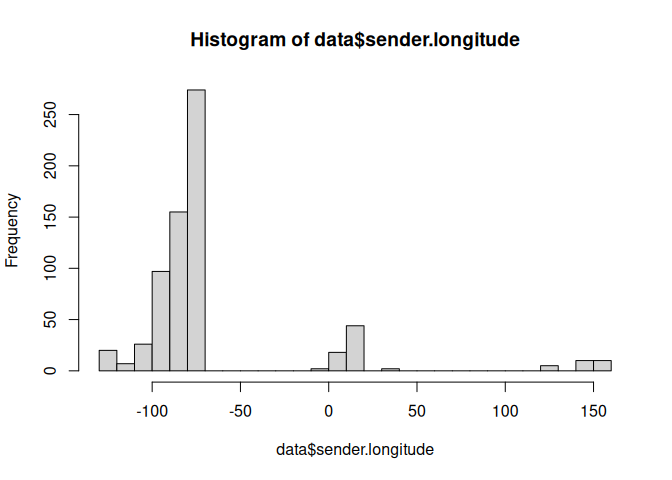
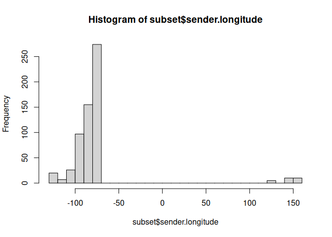
subset <- filter(data, sender.longitude < -50 | sender.longitude > 100)
hist(subset$sender.longitude,breaks=25)
Let’s use the NOT operator to filter out one of the locations.
unique(data$sender.location)
##   [1] "DEU, Mockethal"
##   [2] "USA, St Louis (MS)"
##   [3] "USA, Mobile (AL)"
##   [4] "USA, Laevenworth City (KA)"
##   [5] "USA, Park County (KA)"
##   [6] "USA, Lagrange (TN)"
##   [7] "USA, Cairo (IL)"
##   [8] "USA, Nashville (TN)"
##   [9] "USA, Montgomery (AL)"
##  [10] "USA, Conover (NC)"
##  [11] "USA, Spokane (WA)"
##  [12] "USA, Winona (MN)"
##  [13] "CAN, Dodsland (ON)"
##  [14] "CAN, Hamilton (ON)"
##  [15] "USA, Milwaukee (WI)"
##  [16] "USA, Buffalo (NY)"
##  [17] "DEU, Bremen"
##  [18] "USA, Manitowoc (WI)"
##  [19] "USA, Orange (NJ)"
##  [20] "USA, Cincinnati (OH)"
##  [21] "USA, Newport (KY)"
##  [22] "USA, Oskaloosa (IA)"
##  [23] "USA, Warsaw (IL)"
##  [24] "USA, Koekuk (IA?)"
##  [25] "USA, Maisfeld (near Oskaloosa) (IA)"
##  [26] "DEU, Erfurt"
##  [27] "USA, Detroit (MI)"
##  [28] "DEU, Gotha"
##  [29] "FRA, Versailles"
##  [30] "FRA, Fort de Noisy"
##  [31] "USA, Monroe (MI)"
##  [32] "USA, Tonawanda (NY)"
##  [33] "USA, St. Louis (MO)"
##  [34] "USA, Warschau (IN)"
##  [35] "USA, Oak Grove (WI)"
##  [36] "USA, Edwardsville (IL)"
##  [37] "USA, New York (NY)"
##  [38] "USA, Williamsburg (NY)"
##  [39] "USA, Brooklyn (NY)"
##  [40] "USA, San Francisco (CA)"
##  [41] "CHE,  Amrisweil"
##  [42] "USA, Union Hill (NY)"
##  [43] "USA, Sonoma (CA)"
##  [44] "USA, Richland County (OH)"
##  [45] "USA, New Orleans (LA)"
##  [46] "USA, Dayton (OH)"
##  [47] "DEU, Oberweißbach (TH)"
##  [48] "USA, Waterloo (WI)"
##  [49] "USA, Amherst, Portage Co. (WI)"
##  [50] "USA, Chicago (IL)"
##  [51] "USA, Minneapolis (MN) (MN)"
##  [52] "DEU, Gräfenthal (TH)"
##  [53] "DEU, Piesau (TH)"
##  [54] "USA, Austin (TX)"
##  [55] "USA, Brenham (TX)"
##  [56] "AUS, Sydney"
##  [57] "AUS, Melbourne"
##  [58] "DEU, Hamburg"
##  [59] "BEL, Antwerpen"
##  [60] "DEU, Leipzig (SA)"
##  [61] "AUT, Wien"
##  [62] "AUS, Coolgardie"
##  [63] "AUS, Golden Valley"
##  [64] "AUS, Boulder"
##  [65] "AUS, Moolyelle"
##  [66] "AUS, Waverly"
##  [67] "AUS, Ora Banda"
##  [68] "AUS, Kunanalling"
##  [69] "USA, Walhalla (ND)"
##  [70] "BEL, Antwerpen (Schiff Sorrento)"
##  [71] "GBR, London (Schiff Sorrento)"
##  [72] "EGY, London (Schiff Sorrento)"
##  [73] "AUS, Yougilbar"
##  [74] "AUS, Lionsville"
##  [75] "USA, Cavalier (ND)"
##  [76] "USA, Oliverea (NY)"
##  [77] "USA, Yellowstone (WY)"
##  [78] "USA, Trenton (NJ)"
##  [79] "DEU, Erfurt (TH)"
##  [80] "USA, Perry (OK)"
##  [81] "USA, Shamrock (OK)"
##  [82] "USA, Midford (OK)"
##  [83] "USA, Wellington (KS)"
##  [84] "USA, Rochester (NY)"
##  [85] "USA, Pittsburgh (PN)"
##  [86] "USA, Brownfield (TX)"
##  [87] "USA, Plainview (TX)"
##  [88] "USA, Lubbock (TX)"
##  [89] "USA, Sweetwater (TX)"
##  [90] "USA, Spur (TX)"
##  [91] "USA, Haskell (TX)"
##  [92] "USA, Lamesa (TX)"
##  [93] "USA, Big Spring (TX)"
##  [94] "USA, Seymour (TX)"
##  [95] "USA, Guanah (TX)"
##  [96] "USA, Perryto (TX)"
##  [97] "USA, Burlington (CO)"
##  [98] "USA, Stratton (CO)"
##  [99] "USA, Ozona (TX)"
## [100] "USA, Seminole (TX)"
## [101] "DEU, Jena (TH)"
## [102] "USA, Philadelphia (PA)"
## [103] "DEU, Lobenstein"
## [104] "DEU, Glasin"
## [105] "USA, Cleveland (OH)"
## [106] "USA, Frederick  Maryland"
## [107] "USA, Covington (KY)"
## [108] "USA, Brooko Station"
## [109] "USA, Ohio (OH)"
## [110] "USA, O. Folly Island (SC)"
## [111] "USA, Fernandina (FL)"
## [112] "USA, Jacksonville (FL)"
## [113] "USA, St. Augustine (FL)"
## [114] "DEU, Stuttgart"
## [115] "DEU, Berlin"
## [116] "USA, Blue Ridge Summit (PA)"
## [117] "USA, Warrensville (OH)"
## [118] "USA, Ann Arbor (MI)"
## [119] "USA, Homer (OH)"
## [120] "USA, Wilmington (Delaware)"
## [121] "USA, Columbus (OH)"
## [122] "DEU, München"
## [123] "DEU, Wilhelmshaven"
## [124] "USA, Wood Ridge (NJ)"
## [125] "USA, Jersey City (NJ)"
## [126] "USA, Princeton (NJ)"
## [127] "USA, New York (NY) (NJ)"
## [128] "USA, Port Cester (NY)"
## [129] "USA, Rutherford (NJ)"
## [130] "USA, Carlstadt (NJ)"
## [131] "DEU, Sebnitz (S)"
## [132] "DEU, Eckenhaid"
## [133] "USA, Lime Ridge (WI)"
subset <- filter(data, sender.location != 'USA, Cincinnati (OH)')
unique(subset$sender.location)
##   [1] "DEU, Mockethal"
##   [2] "USA, St Louis (MS)"
##   [3] "USA, Mobile (AL)"
##   [4] "USA, Laevenworth City (KA)"
##   [5] "USA, Park County (KA)"
##   [6] "USA, Lagrange (TN)"
##   [7] "USA, Cairo (IL)"
##   [8] "USA, Nashville (TN)"
##   [9] "USA, Montgomery (AL)"
##  [10] "USA, Conover (NC)"
##  [11] "USA, Spokane (WA)"
##  [12] "USA, Winona (MN)"
##  [13] "CAN, Dodsland (ON)"
##  [14] "CAN, Hamilton (ON)"
##  [15] "USA, Milwaukee (WI)"
##  [16] "USA, Buffalo (NY)"
##  [17] "DEU, Bremen"
##  [18] "USA, Manitowoc (WI)"
##  [19] "USA, Orange (NJ)"
##  [20] "USA, Newport (KY)"
##  [21] "USA, Oskaloosa (IA)"
##  [22] "USA, Warsaw (IL)"
##  [23] "USA, Koekuk (IA?)"
##  [24] "USA, Maisfeld (near Oskaloosa) (IA)"
##  [25] "DEU, Erfurt"
##  [26] "USA, Detroit (MI)"
##  [27] "DEU, Gotha"
##  [28] "FRA, Versailles"
##  [29] "FRA, Fort de Noisy"
##  [30] "USA, Monroe (MI)"
##  [31] "USA, Tonawanda (NY)"
##  [32] "USA, St. Louis (MO)"
##  [33] "USA, Warschau (IN)"
##  [34] "USA, Oak Grove (WI)"
##  [35] "USA, Edwardsville (IL)"
##  [36] "USA, New York (NY)"
##  [37] "USA, Williamsburg (NY)"
##  [38] "USA, Brooklyn (NY)"
##  [39] "USA, San Francisco (CA)"
##  [40] "CHE,  Amrisweil"
##  [41] "USA, Union Hill (NY)"
##  [42] "USA, Sonoma (CA)"
##  [43] "USA, Richland County (OH)"
##  [44] "USA, New Orleans (LA)"
##  [45] "USA, Dayton (OH)"
##  [46] "DEU, Oberweißbach (TH)"
##  [47] "USA, Waterloo (WI)"
##  [48] "USA, Amherst, Portage Co. (WI)"
##  [49] "USA, Chicago (IL)"
##  [50] "USA, Minneapolis (MN) (MN)"
##  [51] "DEU, Gräfenthal (TH)"
##  [52] "DEU, Piesau (TH)"
##  [53] "USA, Austin (TX)"
##  [54] "USA, Brenham (TX)"
##  [55] "AUS, Sydney"
##  [56] "AUS, Melbourne"
##  [57] "DEU, Hamburg"
##  [58] "BEL, Antwerpen"
##  [59] "DEU, Leipzig (SA)"
##  [60] "AUT, Wien"
##  [61] "AUS, Coolgardie"
##  [62] "AUS, Golden Valley"
##  [63] "AUS, Boulder"
##  [64] "AUS, Moolyelle"
##  [65] "AUS, Waverly"
##  [66] "AUS, Ora Banda"
##  [67] "AUS, Kunanalling"
##  [68] "USA, Walhalla (ND)"
##  [69] "BEL, Antwerpen (Schiff Sorrento)"
##  [70] "GBR, London (Schiff Sorrento)"
##  [71] "EGY, London (Schiff Sorrento)"
##  [72] "AUS, Yougilbar"
##  [73] "AUS, Lionsville"
##  [74] "USA, Cavalier (ND)"
##  [75] "USA, Oliverea (NY)"
##  [76] "USA, Yellowstone (WY)"
##  [77] "USA, Trenton (NJ)"
##  [78] "DEU, Erfurt (TH)"
##  [79] "USA, Perry (OK)"
##  [80] "USA, Shamrock (OK)"
##  [81] "USA, Midford (OK)"
##  [82] "USA, Wellington (KS)"
##  [83] "USA, Rochester (NY)"
##  [84] "USA, Pittsburgh (PN)"
##  [85] "USA, Brownfield (TX)"
##  [86] "USA, Plainview (TX)"
##  [87] "USA, Lubbock (TX)"
##  [88] "USA, Sweetwater (TX)"
##  [89] "USA, Spur (TX)"
##  [90] "USA, Haskell (TX)"
##  [91] "USA, Lamesa (TX)"
##  [92] "USA, Big Spring (TX)"
##  [93] "USA, Seymour (TX)"
##  [94] "USA, Guanah (TX)"
##  [95] "USA, Perryto (TX)"
##  [96] "USA, Burlington (CO)"
##  [97] "USA, Stratton (CO)"
##  [98] "USA, Ozona (TX)"
##  [99] "USA, Seminole (TX)"
## [100] "DEU, Jena (TH)"
## [101] "USA, Philadelphia (PA)"
## [102] "DEU, Lobenstein"
## [103] "DEU, Glasin"
## [104] "USA, Cleveland (OH)"
## [105] "USA, Frederick  Maryland"
## [106] "USA, Covington (KY)"
## [107] "USA, Brooko Station"
## [108] "USA, Ohio (OH)"
## [109] "USA, O. Folly Island (SC)"
## [110] "USA, Fernandina (FL)"
## [111] "USA, Jacksonville (FL)"
## [112] "USA, St. Augustine (FL)"
## [113] "DEU, Stuttgart"
## [114] "DEU, Berlin"
## [115] "USA, Blue Ridge Summit (PA)"
## [116] "USA, Warrensville (OH)"
## [117] "USA, Ann Arbor (MI)"
## [118] "USA, Homer (OH)"
## [119] "USA, Wilmington (Delaware)"
## [120] "USA, Columbus (OH)"
## [121] "DEU, München"
## [122] "DEU, Wilhelmshaven"
## [123] "USA, Wood Ridge (NJ)"
## [124] "USA, Jersey City (NJ)"
## [125] "USA, Princeton (NJ)"
## [126] "USA, New York (NY) (NJ)"
## [127] "USA, Port Cester (NY)"
## [128] "USA, Rutherford (NJ)"
## [129] "USA, Carlstadt (NJ)"
## [130] "DEU, Sebnitz (S)"
## [131] "DEU, Eckenhaid"
## [132] "USA, Lime Ridge (WI)"
One handy trick is to select using a list of values.
selected_locations <-c('USA, Brownfield (TX)', 'USA, Rochester (NY)', 'USA, Wellington (KS)')
subset <- filter(data, sender.location %in% selected_locations)
unique(subset$sender.location)
## [1] "USA, Wellington (KS)" "USA, Rochester (NY)" "USA, Brownfield (TX)"
Special cases
Filtering missing values
library(skimr)

# Let's load in a dataset with missing values
pakistan_data <- read_csv("data/pakistan_intellectual_capital.csv")
## New names:
## Rows: 1142 Columns: 13
## ── Column specification
## ──────────────────────────────────────────────────────── Delimiter: "," chr
## (10): Teacher Name, University Currently Teaching, Department, Province ... dbl
## (3): ...1, S#, Year
## ℹ Use `spec()` to retrieve the full column specification for this data. ℹ
## Specify the column types or set `show_col_types = FALSE` to quiet this message.
## • `` -> `...1`
colnames(pakistan_data) <- make.names(colnames(pakistan_data))
skim(pakistan_data)
| Name | pakistan_data |
| Number of rows | 1142 |
| Number of columns | 13 |
| _______________________ | |
| Column type frequency: | |
| character | 10 |
| numeric | 3 |
| ________________________ | |
| Group variables | None |
Data summary
Variable type: character
| skim_variable | n_missing | complete_rate | min | max | empty | n_unique | whitespace |
|---|---|---|---|---|---|---|---|
| Teacher.Name | 0 | 1.00 | 5 | 40 | 0 | 1133 | 0 |
| University.Currently.Teaching | 0 | 1.00 | 7 | 71 | 0 | 63 | 0 |
| Department | 0 | 1.00 | 7 | 43 | 0 | 17 | 0 |
| Province.University.Located | 0 | 1.00 | 3 | 11 | 0 | 5 | 0 |
| Designation | 19 | 0.98 | 4 | 39 | 0 | 46 | 0 |
| Terminal.Degree | 4 | 1.00 | 2 | 30 | 0 | 41 | 0 |
| Graduated.from | 0 | 1.00 | 3 | 88 | 0 | 347 | 0 |
| Country | 0 | 1.00 | 2 | 18 | 0 | 35 | 0 |
| Area.of.Specialization.Research.Interests | 519 | 0.55 | 3 | 477 | 0 | 570 | 0 |
| Other.Information | 1018 | 0.11 | 8 | 132 | 0 | 51 | 0 |
Variable type: numeric
| skim_variable | n_missing | complete_rate | mean | sd | p0 | p25 | p50 | p75 | p100 | hist |
|---|---|---|---|---|---|---|---|---|---|---|
| …1 | 0 | 1.00 | 1054.35 | 520.20 | 2 | 689.25 | 1087.5 | 1476.75 | 1980 | ▅▅▆▇▅ |
| S. | 0 | 1.00 | 1055.35 | 520.20 | 3 | 690.25 | 1088.5 | 1477.75 | 1981 | ▅▅▆▇▅ |
| Year | 653 | 0.43 | 2010.46 | 5.58 | 1983 | 2008.00 | 2012.0 | 2014.00 | 2018 | ▁▁▁▆▇ |
pakistan_data <- drop_na(pakistan_data, Year)
skim(pakistan_data)
| Name | pakistan_data |
| Number of rows | 489 |
| Number of columns | 13 |
| _______________________ | |
| Column type frequency: | |
| character | 10 |
| numeric | 3 |
| ________________________ | |
| Group variables | None |
Data summary
Variable type: character
| skim_variable | n_missing | complete_rate | min | max | empty | n_unique | whitespace |
|---|---|---|---|---|---|---|---|
| Teacher.Name | 0 | 1.00 | 8 | 30 | 0 | 488 | 0 |
| University.Currently.Teaching | 0 | 1.00 | 12 | 55 | 0 | 35 | 0 |
| Department | 0 | 1.00 | 9 | 43 | 0 | 10 | 0 |
| Province.University.Located | 0 | 1.00 | 3 | 11 | 0 | 5 | 0 |
| Designation | 3 | 0.99 | 8 | 39 | 0 | 25 | 0 |
| Terminal.Degree | 0 | 1.00 | 2 | 9 | 0 | 22 | 0 |
| Graduated.from | 0 | 1.00 | 7 | 88 | 0 | 220 | 0 |
| Country | 0 | 1.00 | 2 | 18 | 0 | 25 | 0 |
| Area.of.Specialization.Research.Interests | 170 | 0.65 | 7 | 477 | 0 | 294 | 0 |
| Other.Information | 445 | 0.09 | 8 | 132 | 0 | 23 | 0 |
Variable type: numeric
| skim_variable | n_missing | complete_rate | mean | sd | p0 | p25 | p50 | p75 | p100 | hist |
|---|---|---|---|---|---|---|---|---|---|---|
| …1 | 0 | 1 | 908.79 | 549.68 | 24 | 417 | 892 | 1275 | 1977 | ▇▇▇▅▆ |
| S. | 0 | 1 | 909.79 | 549.68 | 25 | 418 | 893 | 1276 | 1978 | ▇▇▇▅▆ |
| Year | 0 | 1 | 2010.46 | 5.58 | 1983 | 2008 | 2012 | 2014 | 2018 | ▁▁▁▆▇ |
Remove duplicates based on columns
pakistan_data <- read_csv("data/pakistan_intellectual_capital.csv")
## New names:
## Rows: 1142 Columns: 13
## ── Column specification
## ──────────────────────────────────────────────────────── Delimiter: "," chr
## (10): Teacher Name, University Currently Teaching, Department, Province ... dbl
## (3): ...1, S#, Year
## ℹ Use `spec()` to retrieve the full column specification for this data. ℹ
## Specify the column types or set `show_col_types = FALSE` to quiet this message.
## • `` -> `...1`
colnames(pakistan_data) <- make.names(colnames(pakistan_data))
skim(pakistan_data)
| Name | pakistan_data |
| Number of rows | 1142 |
| Number of columns | 13 |
| _______________________ | |
| Column type frequency: | |
| character | 10 |
| numeric | 3 |
| ________________________ | |
| Group variables | None |
Data summary
Variable type: character
| skim_variable | n_missing | complete_rate | min | max | empty | n_unique | whitespace |
|---|---|---|---|---|---|---|---|
| Teacher.Name | 0 | 1.00 | 5 | 40 | 0 | 1133 | 0 |
| University.Currently.Teaching | 0 | 1.00 | 7 | 71 | 0 | 63 | 0 |
| Department | 0 | 1.00 | 7 | 43 | 0 | 17 | 0 |
| Province.University.Located | 0 | 1.00 | 3 | 11 | 0 | 5 | 0 |
| Designation | 19 | 0.98 | 4 | 39 | 0 | 46 | 0 |
| Terminal.Degree | 4 | 1.00 | 2 | 30 | 0 | 41 | 0 |
| Graduated.from | 0 | 1.00 | 3 | 88 | 0 | 347 | 0 |
| Country | 0 | 1.00 | 2 | 18 | 0 | 35 | 0 |
| Area.of.Specialization.Research.Interests | 519 | 0.55 | 3 | 477 | 0 | 570 | 0 |
| Other.Information | 1018 | 0.11 | 8 | 132 | 0 | 51 | 0 |
Variable type: numeric
| skim_variable | n_missing | complete_rate | mean | sd | p0 | p25 | p50 | p75 | p100 | hist |
|---|---|---|---|---|---|---|---|---|---|---|
| …1 | 0 | 1.00 | 1054.35 | 520.20 | 2 | 689.25 | 1087.5 | 1476.75 | 1980 | ▅▅▆▇▅ |
| S. | 0 | 1.00 | 1055.35 | 520.20 | 3 | 690.25 | 1088.5 | 1477.75 | 1981 | ▅▅▆▇▅ |
| Year | 653 | 0.43 | 2010.46 | 5.58 | 1983 | 2008.00 | 2012.0 | 2014.00 | 2018 | ▁▁▁▆▇ |
# Let's check whether the data contains duplicates
# We will assume that people are unique if they have a different terminal degree and graduated from different institutions, and have different names.
pakistan_data <- distinct(pakistan_data, Teacher.Name, Terminal.Degree, Graduated.from)
skim(pakistan_data)
| Name | pakistan_data |
| Number of rows | 1140 |
| Number of columns | 3 |
| _______________________ | |
| Column type frequency: | |
| character | 3 |
| ________________________ | |
| Group variables | None |
Data summary
Variable type: character
| skim_variable | n_missing | complete_rate | min | max | empty | n_unique | whitespace |
|---|---|---|---|---|---|---|---|
| Teacher.Name | 0 | 1 | 5 | 40 | 0 | 1133 | 0 |
| Terminal.Degree | 4 | 1 | 2 | 30 | 0 | 41 | 0 |
| Graduated.from | 0 | 1 | 3 | 88 | 0 | 347 | 0 |
Dropping levels
When you filter data, the factor levels are not automatically dropped.
You can use droplevels() to drop unused levels.
# Creating a demo dataset
animals <- tibble(
  species = factor(c(
    "bat", "bat", "bat",
    "cat", "cat",
    "dog", "dog",
    "fox"
  )),
  habitat = factor(c(
    "cave", "forest", "tree",
    "house", "tree",
    "yard", "house",
    "forest"
  )),
  mass = c(12, 14, 11, 4000, 4100, 15000, 16000, 8000)
)
The tibble stores information about the levels of the factors.
levels(animals$species)
## [1] "bat" "cat" "dog" "fox"
levels(animals$habitat)
## [1] "cave" "forest" "house" "tree" "yard"
Now let’s out the bats.
animals_no_bats <- filter(animals, species != "bat")
levels(animals_no_bats$species)
## [1] "bat" "cat" "dog" "fox"
R keeps all factor levels after filtering because the list of categories represents the full vocabulary of that variable. Removing unused categories would throw away information that might still matter later. It’s easy to remove unused categories but adding that information later is hard. Therefore, the default is to keep it unless you explicitly drop it.
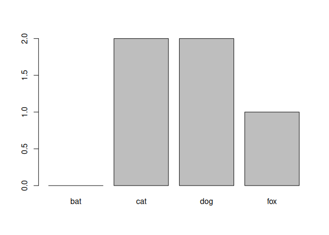
my_table <- table(animals_no_bats$species)
my_table
##
## bat cat dog fox
##   0   2   2   1
barplot(my_table)
Now let’s drop the unused levels.
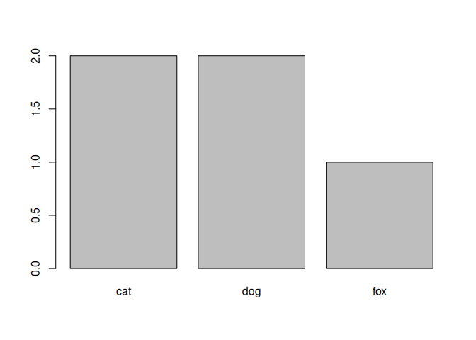
animals_no_bats <- droplevels(animals_no_bats)
levels(animals_no_bats$species)
## [1] "cat" "dog" "fox"
my_table <- table(animals_no_bats$species)
my_table
##
## cat dog fox
##   2   2   1
barplot(my_table)
Ordering rows
You can use arrange to order the rows. Remember that you can also
look at the data using the data viewer in Rstudio. There you can also
sort the data (but this is just the visualization. It does not change
the data itself).
subset1 <-select(data, sender.location, sender.latitude)
subset1 <-arrange(subset1, sender.latitude)
head(subset1, n = 15)
## # A tibble: 15 × 2
##    sender.location    sender.latitude
##    <chr>                        <dbl>
##  1 AUS, Golden Valley           -41.6
##  2 AUS, Golden Valley           -41.6
##  3 AUS, Golden Valley           -41.6
##  4 AUS, Golden Valley           -41.6
##  5 AUS, Golden Valley           -41.6
##  6 AUS, Golden Valley           -41.6
##  7 AUS, Melbourne               -37.8
##  8 AUS, Melbourne               -37.8
##  9 AUS, Moolyelle               -36.8
## 10 AUS, Moolyelle               -36.8
## 11 AUS, Sydney                  -33.9
## 12 AUS, Sydney                  -33.9
## 13 AUS, Sydney                  -33.9
## 14 AUS, Waverly                 -31.9
## 15 AUS, Waverly                 -31.9
Arranging in descending order? No problem.
subset1 <-select(data, sender.location, sender.latitude)
subset1 <-arrange(subset1, desc(sender.latitude))
head(subset1, n = 15)
## # A tibble: 15 × 2
##    sender.location               sender.latitude
##    <chr>                                   <dbl>
##  1 DEU, Glasin                              53.9
##  2 DEU, Glasin                              53.9
##  3 DEU, Glasin                              53.9
##  4 DEU, Hamburg                             53.6
##  5 DEU, Wilhelmshaven                       53.5
##  6 DEU, Wilhelmshaven                       53.5
##  7 DEU, Wilhelmshaven                       53.5
##  8 DEU, Bremen                              53.1
##  9 DEU, Bremen                              53.1
## 10 DEU, Bremen                              53.1
## 11 DEU, Bremen                              53.1
## 12 DEU, Berlin                              52.5
## 13 CAN, Dodsland (ON)                       51.8
## 14 CAN, Dodsland (ON)                       51.8
## 15 GBR, London (Schiff Sorrento)            51.5
Arranging based on multiple columns.
subset1 <-select(data, sender.location, sender.latitude)
subset1 <-mutate(subset1, rounded = round(sender.latitude))
subset1 <-arrange(subset1, desc(rounded), sender.location)
head(subset1, n = 15)
## # A tibble: 15 × 3
##    sender.location               sender.latitude rounded
##    <chr>                                   <dbl>   <dbl>
##  1 DEU, Glasin                              53.9      54
##  2 DEU, Glasin                              53.9      54
##  3 DEU, Glasin                              53.9      54
##  4 DEU, Hamburg                             53.6      54
##  5 DEU, Wilhelmshaven                       53.5      54
##  6 DEU, Wilhelmshaven                       53.5      54
##  7 DEU, Wilhelmshaven                       53.5      54
##  8 DEU, Berlin                              52.5      53
##  9 DEU, Bremen                              53.1      53
## 10 DEU, Bremen                              53.1      53
## 11 DEU, Bremen                              53.1      53
## 12 DEU, Bremen                              53.1      53
## 13 CAN, Dodsland (ON)                       51.8      52
## 14 CAN, Dodsland (ON)                       51.8      52
## 15 GBR, London (Schiff Sorrento)            51.5      52
Exercises
Exercise: Titanic Data
Read in the Titanic.csv data and perform the following operations:
- Count the number of male survivors that were older than 25.
- How many first class passengers were female?
- How many female passengers survived?
Solution
# This set uses two different codes for missing values
titanic_data <- read_csv("data/Titanic.csv", na = c("*", "NA"))
## New names:
## Rows: 1313 Columns: 7
## ── Column specification
## ──────────────────────────────────────────────────────── Delimiter: "," chr
## (3): Name, PClass, Sex dbl (4): ...1, Age, Survived, SexCode
## ℹ Use `spec()` to retrieve the full column specification for this data. ℹ
## Specify the column types or set `show_col_types = FALSE` to quiet this message.
## • `` -> `...1`
# Count the number of male survivors that were older than 25.
# Approach 1
titanic_data_a <- filter(titanic_data, Sex == 'male', Age > 25, Survived == 1)
# Approach 2
titanic_data_b <- filter(titanic_data, Sex == 'male' & Age > 25 & Survived == 1)


# How many first class passengers were female?
# Approach 1
titanic_data_c <- filter(titanic_data, PClass == '1st', Sex == 'female')
# Approach 2
titanic_data_d <- filter(titanic_data, PClass == '1st' & Sex == 'female')

# How many female passengers survived?
# Approach 1
titanic_data_e <- filter(titanic_data, Sex == 'female', Survived == 1)
# Approach 2
titanic_data_f <- filter(titanic_data, Sex == 'female' & Survived == 1)
Exercise: Car data
Read in the cars.txt data and perform the following operations:
The data file contains variables describing a number of cars.
- Select all cars with at least 25 mpg in the city.
- Select all BMW’s
- Are there any Large cars with more than 25 mpg in the city?
- Which cars use over 50% more fuel on the city than they do in the highway?
- Which cars have an action radius of over 400 miles on the highway?
Solution
car_data <- read_delim("data/cars.txt", delim = " ")
## Rows: 93 Columns: 26
## ── Column specification ────────────────────────────────────────────────────────
## Delimiter: " "
## chr  (6): make, model, type, cylinders, rearseat, luggage
## dbl (20): min_price, mid_price, max_price, mpg_city, mpg_hgw, airbag, drive,...
##
## ℹ Use `spec()` to retrieve the full column specification for this data.
## ℹ Specify the column types or set `show_col_types = FALSE` to quiet this message.
selection_a <- filter(car_data, mpg_city >= 25)
selection_b <- filter(car_data, make == 'BMW')
selection_c <- filter(car_data, mpg_city >= 25, type=='Large')

selection_d <- filter(car_data, mpg_city > 1.5*mpg_hgw)

car_data <- mutate(car_data, action_radius = tank * mpg_hgw)
selection_e <- filter(car_data, action_radius > 400)
Exercise: Film data
Use the following data file: films.dat (in the data folder). This file
lists the title, year of release, length in minutes, number of cast
members listed, rating, and number of lines of description are recorded
for a simple random sample of 100 movies.
-
Write code to select all films from 1980 to 1990 (including both 1980 and 1990)
-
Select all films with a rating of 1
-
Write a short script that allows selecting all movies that were made in the five years before a given date. The script starts by assigning a value (year) to a variable. The script selects all movies made in the 5 years preceding the year assigned to the variable and prints the selected data to the screen. The earliest film in the data was made in 1924. Therefore, if the year assigned to the variable is before 1930, the script should print the message
No movies found. -
Write code that adds a new variable
ratioto the data. This variable is obtained by dividing the number of actors (Cast) by the length of the movie (Length). Next, select the movies for which the ratio Cast/Length is at least 0.1. Print the selected movies to the screen.
Solution
# The data uses a tab as a delimiter
film_data <- read_delim("data/films.dat", delim = "\t")
## Rows: 100 Columns: 6
## ── Column specification ────────────────────────────────────────────────────────
## Delimiter: "\t"
## chr (1): Title
## dbl (5): Year, Length, Cast, Rating, Description
##
## ℹ Use `spec()` to retrieve the full column specification for this data.
## ℹ Specify the column types or set `show_col_types = FALSE` to quiet this message.
# select all films from 1980 to 1990 (including both 1980 and 1990)
selection_a <- filter(film_data, Year >= 1980 & Year <= 1990)

# select all films with a rating of 1
selection_b <- filter(film_data, Rating == 1)

# Select films made in the five years before a given date
selected_year <- 1980
film_data <- mutate(film_data, too_old = Year - selected_year < -5)
film_data <- mutate(film_data, too_new = Year - selected_year > 0)
selected_films <- filter(film_data, !too_old & !too_new)
nr_selected <- dim(selected_films)[1]
if (nr_selected == 0) {
  print("No movies found")
} else {
  print(paste("Number of movies found:", nr_selected))
}
## [1] "Number of movies found: 12"
# Add a new variable ratio to the data
film_data <- mutate(film_data, ratio = Cast / Length)
selection_c <- filter(film_data, ratio >= 0.1)