Reading Data
Last Updated: 18, November, 2025 at 08:27
- Before we begin…
- Using the tidyverse vs built-in data reading functions
- Reading data from excel using readxl
- Reading data from a comma separated text file
- Dealing with file not found errors
- Tibbles
- Some interesting options when using
read_csv() - Reading files not separated by commas
- Exploring data
- Addressing a single variable
- Creating new variables
- Creating new variables using
mutate - Exercises
- Possible solutions
library(tidyverse)
## ── Attaching core tidyverse packages ──────────────────────── tidyverse 2.0.0 ──
## ✔ dplyr     1.1.4     ✔ readr     2.1.5
## ✔ forcats   1.0.1     ✔ stringr   1.5.2
## ✔ ggplot2   4.0.0     ✔ tibble    3.3.0
## ✔ lubridate 1.9.4     ✔ tidyr     1.3.1
## ✔ purrr     1.1.0
## ── Conflicts ────────────────────────────────────────── tidyverse_conflicts() ──
## ✖ dplyr::filter() masks stats::filter()
## ✖ dplyr::lag()    masks stats::lag()
## ℹ Use the conflicted package (<http://conflicted.r-lib.org/>) to force all conflicts to become errors
Before we begin…
Download the following data files to your computer from the
GradStats > Data Wrangling > Data.
transit-data.xlsxpakistan_intellectual_capital.csvcars.txtwages1833.csv
Using the tidyverse vs built-in data reading functions
Default function
In base R, the default function for reading tabular data from a CSV file
is read.csv(). This function is widely used, but it has some quirks:
-
Automatic conversion of strings to factors (before R version 4.0.0): By default,
read.csv()automatically converts character columns to factors, which can cause issues if you’re not expecting categorical data. You can disable this behavior by settingstringsAsFactors = FALSE. -
Column name handling: Column names are automatically adjusted to be syntactically valid variable names. For example, spaces are replaced with periods (.), which can make column names harder to read.
-
Performance: While
read.csv()is perfectly fine for smaller datasets, it can be slower when working with larger files.
Example usage:
data <- read.csv("data/pakistan_intellectual_capital.csv")
The tidyverse way
The tidyverse provides its own functions to read data. For example, the
nearly-equivalent function to read.csv() is read_csv() (from the
readr package). Notice the small difference in the function name!
The tidyverse provides a more user-friendly function for reading CSV
files: read_csv() from the readr package. It addresses many of the
limitations of read.csv() and offers a more intuitive experience for
modern data analysis:
- Type guessing:
read_csv()automatically guesses the types of columns (e.g., numeric, character, date) but does not convert them to factors unless specified. - Handling of column names: Column names are left as-is, without modification. This keeps names readable, especially when they contain spaces or special characters.
- Faster performance:
read_csv()is optimized for speed and can handle larger datasets more efficiently thanread.csv(). This performance difference becomes noticeable for very large datasets (e.g., over 1 GB). - Tibble output: The result of
read_csv()is a tibble, which has advantages over a data.frame, such as better printing in the console and more intuitive column subsetting.
Example usage:
data <- read_csv("data/pakistan_intellectual_capital.csv")
## New names:
## Rows: 1142 Columns: 13
## ── Column specification
## ──────────────────────────────────────────────────────── Delimiter: "," chr
## (10): Teacher Name, University Currently Teaching, Department, Province ... dbl
## (3): ...1, S#, Year
## ℹ Use `spec()` to retrieve the full column specification for this data. ℹ
## Specify the column types or set `show_col_types = FALSE` to quiet this message.
## • `` -> `...1`
This is just a quick example. We’ll look more at how to read in data from CSV below. Throughout this class, I will try to use the tidyverse functions for reading data.
Note on paths
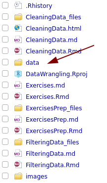
Since we’re working with in a RStudio Project, your working
directory is automatically set to your project folder. This makes
managing file paths much simpler! In this case, I assume you organized
your project with the following structure (the project name MyRProject
can differ):
MyRProject/
├── MyRProject.Rproj
├── data/
│   ├── transit-data.xlsx
│   ├── pakistan_intellectual_capital.csv
│   ├── cars.txt
│   └── wages1833.csv
├── scripts/
└── output/
R will still find the files as long as you use paths relative to your
project folder. This means you can place your scripts in a separate
scripts/ folder and your data in a data/ folder without any issues.
You could also keep the scripts and data in the top folder.
You can verify where R is looking for files using:
getwd()
## [1] "/home/dieter/Dropbox/GraduateStatistics/GradStats/02 Data Wrangling"
With your data organized in a data/ folder, you can use relative
paths to read files. The path is “relative” because it’s relative to
your project folder. When you share your project with others or move it
to a different computer, the code will still work as long as the folder
structure stays the same.
# This looks for the 'data' folder inside your project directory
data <- read_csv("data/pakistan_intellectual_capital.csv")
Note on file path separators
R accepts forward slashes (/) in file paths on all operating systems,
including Windows. This is the recommended approach for cross-platform
compatibility:
"data/myfile.csv"(works everywhere - use this!)"data\\myfile.csv"(works on Windows with escaped backslash, but unnecessary)"data\myfile.csv"(causes errors -\is an escape character)
Bottom line: Always use forward slashes in your R code, even on Windows.
Reading data from excel using readxl
Excel spreadsheets are often used and easy way to store data.
Explore the data in transit-data.xlsx. (Please note the organization
of my project folder.)
Note that:
- The data do not start in cell A1
- The data contain different date formats
- The data contain weird characters
Read the first sheet of data:
library(readxl)
data <-read_excel("data/transit-data.xlsx") #Be sure to use the correct relative path here.
Look at the help for the read_excel function:
#Let's specify the data range we want to read.
info <-read_excel("data/transit-data.xlsx", sheet = 'info', range = 'B1:C7')
info <-read_excel("data/transit-data.xlsx", sheet = 'info', range = cell_cols('B:C'))
Let’s now read the data in the second sheet:
more_data <- read_excel("data/transit-data.xlsx", sheet = 'transport data')
## New names:
## • `` -> `...2`
## • `` -> `...3`
## • `` -> `...5`
## • `` -> `...6`
## • `` -> `...8`
We need to skip the first line of the data.
more_data <- read_excel("data/transit-data.xlsx", sheet = 'transport data', skip=1)
The column names are human readable but not very handy for coding. There is a quick way to solve this.
Pro Tip: Only use underscores or dots in column names. This will make your life easier when coding.
more_data <- read_excel("data/transit-data.xlsx", sheet = 'transport data', skip=1)
colnames(more_data)
## [1] "sender location"    "sender latitude"    "sender longitude"
## [4] "receiver location"  "receiver latitude"  "receiver longitude"
## [7] "date"               "number of items"
colnames(more_data) <- make.names(colnames(more_data))
colnames(more_data)
## [1] "sender.location"    "sender.latitude"    "sender.longitude"
## [4] "receiver.location"  "receiver.latitude"  "receiver.longitude"
## [7] "date"               "number.of.items"
Another, more modern, way to do this is using the janitor package (we
will use this package again below).
library(janitor)
##
## Attaching package: 'janitor'

## The following objects are masked from 'package:stats':
##
##     chisq.test, fisher.test
more_data <- read_excel("data/transit-data.xlsx", sheet = 'transport data', skip=1)
names(more_data)
## [1] "sender location"    "sender latitude"    "sender longitude"
## [4] "receiver location"  "receiver latitude"  "receiver longitude"
## [7] "date"               "number of items"
names(more_data) <- make_clean_names(names(more_data))
names(more_data)
## [1] "sender_location"    "sender_latitude"    "sender_longitude"
## [4] "receiver_location"  "receiver_latitude"  "receiver_longitude"
## [7] "date"               "number_of_items"
Reading data from a comma separated text file
R has functions for reading in text files. However, the functions provided by tidyverse are often more powerful. When reading in data, R reports on the column types. Information about the different types and their labels can be found here: Column Types
Note: The default report on the column types is a bit disorganized in this view. It will look better in your console.
data <- read_csv('data/pakistan_intellectual_capital.csv')
## New names:
## Rows: 1142 Columns: 13
## ── Column specification
## ──────────────────────────────────────────────────────── Delimiter: "," chr
## (10): Teacher Name, University Currently Teaching, Department, Province ... dbl
## (3): ...1, S#, Year
## ℹ Use `spec()` to retrieve the full column specification for this data. ℹ
## Specify the column types or set `show_col_types = FALSE` to quiet this message.
## • `` -> `...1`
# The read functions in the tidyverse are trying to be helpful by printing some output about the how the data was interpreted during reading. If you don't like the output, you can switch this off.
# Now the function only reports it has 'repaired` a variable name.
data <- read_csv('data/pakistan_intellectual_capital.csv', show_col_types = FALSE)
## New names:
## • `` -> `...1`
Note that this file has stray line endings that look like empty lines. This explains why the datafile has 1236 lines but the data read in has only 1142 lines.

You can check whether there were any problems during reading the data
using the problems() function. In this case, no problems are reported.
# Check for problems
probs <- problems(data)
print(probs)
## # A tibble: 0 × 5
## # ℹ 5 variables: row <int>, col <int>, expected <chr>, actual <chr>, file <chr>
Dealing with file not found errors
When reading in data, you might encounter a “file not found” error. This means that R cannot locate the file at the specified path. Here are some steps to troubleshoot and resolve this issue.
Step 1: Get the absolute path of the file you want to read
What is an absolute path?
An absolute path is the full, exact location of a file or folder on your computer. It starts at the very top of the file system and includes every folder along the way, all the way down to the file itself.
On Windows, an absolute path always begins with a drive letter such as
C:. For example:
C:\Users\yourname\Documents\Data\birds.csv
On macOS and Linux/Unix-like systems, there are no drive letters.
Instead, an absolute path always starts with a leading slash /, which
represents the root of the entire file system. For example:
/Users/yourname/Documents/Data/birds.csv
Getting the absolute path of the file in Windows
- Open File Explorer and find your file.
- Hold Shift, then right-click the file.
- Choose “Copy as path”.
- Paste into notepad. This will show the absolute path of the file.
Keep the file open. You will need it in step 3.
Getting the absolute path of the file on Mac
- Open Finder and locate your file.
- Right-click the file.
- Hold the Option (⌥) key — this reveals extra menu options.
- Click “Copy (filename) as Pathname”.
- Paste into a text editor (e.g., TextEdit). This will show the absolute path of the file.
Keep the file open. You will need it in step 3.
Step 2: Get the absolute path of the file you want to read as R interprets it
You can use path_abs() to have R print the absolute path of the file
you are trying to read, even if that path does not exist on your
computer. This shows you exactly what R is trying to do and where it is
looking.
For example, suppose you are trying to run:
data <- read_csv("Data/Birds.csv") # Here "Data/Birds.csv" is a relative path.
To see the absolute path R is using, run the following in the R console:
library(fs)
path_in_r <- "Data/Birds.csv"   # Replace this with the path you are using
path_abs(path_in_r)
For windows, R might print something like:
C:/Users/yourname/Documents/StatsClass/Data/Birds.csv
On macOS, you would get something like:
/Users/yourname/Documents/StatsClass/Data/Birds.csv
Copy the result to the same text file you copied the absolute path file to before.
Bonus hint
You can including the following snippet of code in your script to automatically print the absolute path R is using when you try to read a file. This can be very helpful for debugging.
library(fs) # You need to load the fs library to use this trick
path_in_r <- "Data/Birds.csv"   # Replace this with the path you are using
print(path_abs(path_in_r)) # Print the path where R will be looking for the file
data <- read_csv(path_in_r) # Now read in the file
If R says it can’t find the file, take a look at the output of the print statement to see where R is looking for the file.
Step 3: Compare the two paths
- The first path you copied to the text editor is the place where the file actually lives.
- The second path (from
path_abs()) is the place where R is looking for the file.
If the two paths are not 100% identical, R will not be able to find the file.
Common issues to check:
-
Working directory:
If you used a relative path in R, is R using the correct working directory?
You can reset the working directory to the project’s directory using:
Session > Set Working Directory > To Project Directory. -
Spelling and capitalization:
Are there any spelling mistakes in the path you wrote in R?
Does the capitalization match the actual file name and folder names?
(macOS and Linux are case-sensitive.) -
Spaces in folder names:
Does your path contain spaces (e.g.,My Documents,Stats Class,Week 1)?
Make sure the entire path is wrapped in quotes in your R code**:
"My Documents/Stats Class/Week 1/birds.csv".
Without quotes, R will treat a space as the end of the file name.
Tibbles
Reading in data using tidyverse functions generates tibbles, instead
of R’s traditional data.frame. These are a newer version of the
classic data frame with features tweaked to make life a bit easier.
- Printing: Tibbles print more concisely than
data.frames. They show a preview of the data, while data.frames show the entire dataset in the console. - Subsetting: When you subset a data.frame with
mydata[1], the result is still a data.frame, whereas in a tibble, subsetting a column withmydata[[1]]ormydata$column_namereturns a vector directly. See tabke below. - Casting: Tibbles preserve the type of data you provide. A
data.frame, might coerce data into factors.
print(class(data))
## [1] "spec_tbl_df" "tbl_df" "tbl" "data.frame"
Convert to an old school data frame.
old_school<-as.data.frame(data)
Some interesting options when using read_csv()
No column names? No problem!
If data has no column names, use col_names = FALSE
read_csv("1,2,3\n4,5,6", col_names = FALSE)
## Rows: 2 Columns: 3
## ── Column specification ────────────────────────────────────────────────────────
## Delimiter: ","
## dbl (3): X1, X2, X3
##
## ℹ Use `spec()` to retrieve the full column specification for this data.
## ℹ Specify the column types or set `show_col_types = FALSE` to quiet this message.

## # A tibble: 2 × 3
##      X1    X2    X3
##   <dbl> <dbl> <dbl>
## 1     1     2     3
## 2     4     5     6
You can also directly set the column names in this case.
read_csv("1,2,3\n4,5,6", col_names = c("x", "y", "z"))
## Rows: 2 Columns: 3
## ── Column specification ────────────────────────────────────────────────────────
## Delimiter: ","
## dbl (3): x, y, z
##
## ℹ Use `spec()` to retrieve the full column specification for this data.
## ℹ Specify the column types or set `show_col_types = FALSE` to quiet this message.

## # A tibble: 2 × 3
##       x     y     z
##   <dbl> <dbl> <dbl>
## 1     1     2     3
## 2     4     5     6
Specifying missing data
Another option that commonly needs tweaking is na: this specifies the
value (or values) that are used to represent missing values in your
file:
read_csv("a,b,c\n1,2,.", na = ".")
## Rows: 1 Columns: 3
## ── Column specification ────────────────────────────────────────────────────────
## Delimiter: ","
## dbl (2): a, b
## lgl (1): c
##
## ℹ Use `spec()` to retrieve the full column specification for this data.
## ℹ Specify the column types or set `show_col_types = FALSE` to quiet this message.

## # A tibble: 1 × 3
##       a     b c
##   <dbl> <dbl> <lgl>
## 1     1     2 NA
You can also specify multiple values that should be considered as missing data.
data <- read_csv("a,b,c\n1,2,.\n5,6,NA\n8,0,1", na = c("NA", "."))
## Rows: 3 Columns: 3
## ── Column specification ────────────────────────────────────────────────────────
## Delimiter: ","
## dbl (3): a, b, c
##
## ℹ Use `spec()` to retrieve the full column specification for this data.
## ℹ Specify the column types or set `show_col_types = FALSE` to quiet this message.
head(data)
## # A tibble: 3 × 3
##       a     b     c
##   <dbl> <dbl> <dbl>
## 1     1     2    NA
## 2     5     6    NA
## 3     8     0     1
Reading from URL
You can read data directly from a URL as well.
url<-'https://raw.githubusercontent.com/dvanderelst-python-class/python-class/fall2022/11_Pandas_Statistics/data/pizzasize.csv'
data <- read_csv(url)
## Rows: 250 Columns: 5
## ── Column specification ────────────────────────────────────────────────────────
## Delimiter: ","
## chr (3): Store, CrustDescription, Topping
## dbl (2): ID, Diameter
##
## ℹ Use `spec()` to retrieve the full column specification for this data.
## ℹ Specify the column types or set `show_col_types = FALSE` to quiet this message.
Getting rid of that pesky index column
Many datasets have a first column that is some index. This is typically not needed. And sometimes, these aren’t given names in the data file. Here is a way to avoid reading these in.
data <- read_csv('data/pakistan_intellectual_capital.csv')
## New names:
## Rows: 1142 Columns: 13
## ── Column specification
## ──────────────────────────────────────────────────────── Delimiter: "," chr
## (10): Teacher Name, University Currently Teaching, Department, Province ... dbl
## (3): ...1, S#, Year
## ℹ Use `spec()` to retrieve the full column specification for this data. ℹ
## Specify the column types or set `show_col_types = FALSE` to quiet this message.
## • `` -> `...1`
names(data)
##  [1] "...1"
##  [2] "S#"
##  [3] "Teacher Name"
##  [4] "University Currently Teaching"
##  [5] "Department"
##  [6] "Province University Located"
##  [7] "Designation"
##  [8] "Terminal Degree"
##  [9] "Graduated from"
## [10] "Country"
## [11] "Year"
## [12] "Area of Specialization/Research Interests"
## [13] "Other Information"
# Don't read the first column
data <- read_csv('data/pakistan_intellectual_capital.csv', col_select = -1)
## New names:
## Rows: 1142 Columns: 12
## ── Column specification
## ──────────────────────────────────────────────────────── Delimiter: "," chr
## (10): Teacher Name, University Currently Teaching, Department, Province ... dbl
## (2): S#, Year
## ℹ Use `spec()` to retrieve the full column specification for this data. ℹ
## Specify the column types or set `show_col_types = FALSE` to quiet this message.
## • `` -> `...1`
names(data)
##  [1] "S#"
##  [2] "Teacher Name"
##  [3] "University Currently Teaching"
##  [4] "Department"
##  [5] "Province University Located"
##  [6] "Designation"
##  [7] "Terminal Degree"
##  [8] "Graduated from"
##  [9] "Country"
## [10] "Year"
## [11] "Area of Specialization/Research Interests"
## [12] "Other Information"
Reading files not separated by commas
read_csv() expects comma separated field. For data separated by other
characters use these:
read_table()reads files with white space as the delimiter. It also handles ragged data.- all others:
read_delim(), specifying thedelimargument. read_csv2()uses;for the field separator and,for the decimal point. This format is common in some European countries.
Exploring data
After reading in the data, it’s a good idea to explore the data. Use either the environment tab in Rstudio or use functions that give you some info about your data.
“This is a critical step that should always be performed. It is simple but it is vital. You should make numerical summaries such as means, standard deviations (SDs), maximum and minimum, correlations and whatever else is appropriate to the specific dataset. Equally important are graphical summaries.”
(Faraway, J. J. (2004). Linear models with R. Chapman and Hall/CRC.).
One of the most simple things you can do is inspect your data using a text editor. When text files are large, it’s a good idea to get an editor that can handle large files. I suggest Sublime Text Editor. This editor can handle much larger files than you can open (as text) in Rstudio. Keep the file open while you’re cleaning it!
There are many text editors out there. Shop around and find one you like. Some other suggestions:
- Notepad++ (Windows only)
- Visual Studio Code (cross-platform)
- BBEdit (Mac only)
- Geany (cross-platform, lightweight)
Let’s read in some data:
data <- read_csv('data/pakistan_intellectual_capital.csv')
## New names:
## Rows: 1142 Columns: 13
## ── Column specification
## ──────────────────────────────────────────────────────── Delimiter: "," chr
## (10): Teacher Name, University Currently Teaching, Department, Province ... dbl
## (3): ...1, S#, Year
## ℹ Use `spec()` to retrieve the full column specification for this data. ℹ
## Specify the column types or set `show_col_types = FALSE` to quiet this message.
## • `` -> `...1`
Column names
names(data)
##  [1] "...1"
##  [2] "S#"
##  [3] "Teacher Name"
##  [4] "University Currently Teaching"
##  [5] "Department"
##  [6] "Province University Located"
##  [7] "Designation"
##  [8] "Terminal Degree"
##  [9] "Graduated from"
## [10] "Country"
## [11] "Year"
## [12] "Area of Specialization/Research Interests"
## [13] "Other Information"
Head and tail
head(data)
## # A tibble: 6 × 13
##    ...1  `S#` `Teacher Name`      `University Currently Teaching`     Department
##   <dbl> <dbl> <chr>               <chr>                               <chr>
## 1     2     3 Dr. Abdul Basit     University of Balochistan           Computer …
## 2     4     5 Dr. Waheed Noor     University of Balochistan           Computer …
## 3     5     6 Dr. Junaid Baber    University of Balochistan           Computer …
## 4     6     7 Dr. Maheen Bakhtyar University of Balochistan           Computer …
## 5    24    25 Samina Azim         Sardar Bahadur Khan Women's Univer… Computer …
## 6    25    26 Nausheed Saeed      Sardar Bahadur Khan Women's Univer… Computer …
## # ℹ 8 more variables: `Province University Located` <chr>, Designation <chr>,
## #   `Terminal Degree` <chr>, `Graduated from` <chr>, Country <chr>, Year <dbl>,
## #   `Area of Specialization/Research Interests` <chr>,
## #   `Other Information` <chr>
tail(data)
## # A tibble: 6 × 13
##    ...1  `S#` `Teacher Name`         `University Currently Teaching` Department
##   <dbl> <dbl> <chr>                  <chr>                           <chr>
## 1  1971  1972 Dr. Khalid J Siddiqui  Ghulam Ishaq Khan Institute     Computer S…
## 2  1974  1975 Dr. Ahmar Rashid       Ghulam Ishaq Khan Institute     Computer S…
## 3  1975  1976 Dr. Fawad Hussain      Ghulam Ishaq Khan Institute     Computer S…
## 4  1977  1978 Dr. Rashad M Jillani   Ghulam Ishaq Khan Institute     Computer S…
## 5  1979  1980 Dr. Shahabuddin Ansari Ghulam Ishaq Khan Institute     Computer S…
## 6  1980  1981 Dr. Sajid Anwar        Ghulam Ishaq Khan Institute     Computer S…
## # ℹ 8 more variables: `Province University Located` <chr>, Designation <chr>,
## #   `Terminal Degree` <chr>, `Graduated from` <chr>, Country <chr>, Year <dbl>,
## #   `Area of Specialization/Research Interests` <chr>,
## #   `Other Information` <chr>
Summary
Get a quick summary
summary(data)
##       ...1              S#         Teacher Name
##  Min.   :   2.0   Min.   :   3.0   Length:1142
##  1st Qu.: 689.2   1st Qu.: 690.2   Class :character
##  Median :1087.5   Median :1088.5   Mode  :character
##  Mean   :1054.4   Mean   :1055.4
##  3rd Qu.:1476.8   3rd Qu.:1477.8
##  Max.   :1980.0   Max.   :1981.0
##
##  University Currently Teaching  Department        Province University Located
##  Length:1142                   Length:1142        Length:1142
##  Class :character              Class :character   Class :character
##  Mode  :character              Mode  :character   Mode  :character
##
##
##
##
##  Designation        Terminal Degree    Graduated from       Country
##  Length:1142        Length:1142        Length:1142        Length:1142
##  Class :character   Class :character   Class :character   Class :character
##  Mode  :character   Mode  :character   Mode  :character   Mode  :character
##
##
##
##
##       Year      Area of Specialization/Research Interests Other Information
##  Min.   :1983   Length:1142                               Length:1142
##  1st Qu.:2008   Class :character                          Class :character
##  Median :2012   Mode  :character                          Mode  :character
##  Mean   :2010
##  3rd Qu.:2014
##  Max.   :2018
##  NA's   :653
Glimpse
The function glimpse gives you also a quick overview:
glimpse(data)
## Rows: 1,142
## Columns: 13
## $ ...1                                        <dbl> 2, 4, 5, 6, 24, 25, 26, 27…
## $ `S#`                                        <dbl> 3, 5, 6, 7, 25, 26, 27, 28…
## $ `Teacher Name`                              <chr> "Dr. Abdul Basit", "Dr. Wa…
## $ `University Currently Teaching`             <chr> "University of Balochistan…
## $ Department                                  <chr> "Computer Science & IT", "…
## $ `Province University Located`               <chr> "Balochistan", "Balochista…
## $ Designation                                 <chr> "Assistant Professor", "As…
## $ `Terminal Degree`                           <chr> "PhD", "PhD", "PhD", "PhD"…
## $ `Graduated from`                            <chr> "Asian Institute of Techno…
## $ Country                                     <chr> "Thailand", "Thailand", "T…
## $ Year                                        <dbl> NA, NA, NA, NA, 2005, 2008…
## $ `Area of Specialization/Research Interests` <chr> "Software Engineering & DB…
## $ `Other Information`                         <chr> NA, NA, NA, NA, NA, NA, NA…
Skim
And what about this beautiful exploratory tool?
library(skimr)
skim(data)
| Name | data |
| Number of rows | 1142 |
| Number of columns | 13 |
| _______________________ | |
| Column type frequency: | |
| character | 10 |
| numeric | 3 |
| ________________________ | |
| Group variables | None |
Data summary
Variable type: character
| skim_variable | n_missing | complete_rate | min | max | empty | n_unique | whitespace |
|---|---|---|---|---|---|---|---|
| Teacher Name | 0 | 1.00 | 5 | 40 | 0 | 1133 | 0 |
| University Currently Teaching | 0 | 1.00 | 7 | 71 | 0 | 63 | 0 |
| Department | 0 | 1.00 | 7 | 43 | 0 | 17 | 0 |
| Province University Located | 0 | 1.00 | 3 | 11 | 0 | 5 | 0 |
| Designation | 19 | 0.98 | 4 | 39 | 0 | 46 | 0 |
| Terminal Degree | 4 | 1.00 | 2 | 30 | 0 | 41 | 0 |
| Graduated from | 0 | 1.00 | 3 | 88 | 0 | 347 | 0 |
| Country | 0 | 1.00 | 2 | 18 | 0 | 35 | 0 |
| Area of Specialization/Research Interests | 519 | 0.55 | 3 | 477 | 0 | 570 | 0 |
| Other Information | 1018 | 0.11 | 8 | 132 | 0 | 51 | 0 |
Variable type: numeric
| skim_variable | n_missing | complete_rate | mean | sd | p0 | p25 | p50 | p75 | p100 | hist |
|---|---|---|---|---|---|---|---|---|---|---|
| …1 | 0 | 1.00 | 1054.35 | 520.20 | 2 | 689.25 | 1087.5 | 1476.75 | 1980 | ▅▅▆▇▅ |
| S# | 0 | 1.00 | 1055.35 | 520.20 | 3 | 690.25 | 1088.5 | 1477.75 | 1981 | ▅▅▆▇▅ |
| Year | 653 | 0.43 | 2010.46 | 5.58 | 1983 | 2008.00 | 2012.0 | 2014.00 | 2018 | ▁▁▁▆▇ |
skim_tee(data)
## ── Data Summary ────────────────────────
##                            Values
## Name                       data
## Number of rows             1142
## Number of columns          13
## _______________________
## Column type frequency:
##   character                10
##   numeric                  3
## ________________________
## Group variables            None
##
## ── Variable type: character ────────────────────────────────────────────────────
##    skim_variable                             n_missing complete_rate min max
##  1 Teacher Name                                      0         1       5  40
##  2 University Currently Teaching                     0         1       7  71
##  3 Department                                        0         1       7  43
##  4 Province University Located                       0         1       3  11
##  5 Designation                                      19         0.983   4  39
##  6 Terminal Degree                                   4         0.996   2  30
##  7 Graduated from                                    0         1       3  88
##  8 Country                                           0         1       2  18
##  9 Area of Specialization/Research Interests       519         0.546   3 477
## 10 Other Information                              1018         0.109   8 132
##    empty n_unique whitespace
##  1     0     1133          0
##  2     0       63          0
##  3     0       17          0
##  4     0        5          0
##  5     0       46          0
##  6     0       41          0
##  7     0      347          0
##  8     0       35          0
##  9     0      570          0
## 10     0       51          0
##
## ── Variable type: numeric ──────────────────────────────────────────────────────
##   skim_variable n_missing complete_rate  mean     sd   p0   p25   p50   p75 p100
## 1 ...1                  0         1     1054. 520.      2  689. 1088. 1477. 1980
## 2 S#                    0         1     1055. 520.      3  690. 1088. 1478. 1981
## 3 Year                653         0.428 2010.   5.58 1983 2008  2012  2014  2018
##   hist
## 1 ▅▅▆▇▅
## 2 ▅▅▆▇▅
## 3 ▁▁▁▆▇
Tabulating
You can use the janitor package to get a quick overview of categorical
variables, i.e., tabulating categorical variables. It’s somewhat
confusing that the percent column is not a percentage but a
proportion.
library(janitor)
tabyl(data, `Province University Located`)
##  Province University Located   n    percent
##                  Balochistan  16 0.01401051
##                      Capital 247 0.21628722
##                          KPK  86 0.07530648
##                       Punjab 449 0.39316988
##                        Sindh 344 0.30122592
Addressing a single variable
A simple way to get variables from a tibble is using the $ operator.
my_variable <- data$Year
summary(my_variable)
##    Min. 1st Qu.  Median    Mean 3rd Qu.    Max.    NA's
##    1983    2008    2012    2010    2014    2018     653
However, this does not work if your variables names have names with a space (or other weird characters). This does work, however,
my_variable <- data['Terminal Degree']
This table gives some more details about variables can be addressed.
| Expression | Works | Returns / Behavior |
|---|---|---|
data$Year |
Yes | Column vector |
data[["Year"]] |
Yes | Column vector |
data["Year"] |
Yes | One-column data.frame / tibble |
data$Terminal Degree |
No | Error: space in name — not syntactically valid |
data$'Terminal Degree' |
No | Error: quotes not allowed after $ |
data$"Terminal Degree" |
No | Error: same as above |
data[terminal degree] |
No | Error: object ‘terminal’ not found — needs quotes |
data[["Terminal Degree"]] |
Yes | Column vector |
data["Terminal Degree"] |
Yes | One-column data.frame / tibble |
Creating new variables
Often, you will want to create new variables based on existing ones to make subsequent processing easier.
data['very_simple'] <- 1
data['very_simple']
## # A tibble: 1,142 × 1
##    very_simple
##          <dbl>
##  1           1
##  2           1
##  3           1
##  4           1
##  5           1
##  6           1
##  7           1
##  8           1
##  9           1
## 10           1
## # ℹ 1,132 more rows
However, we can do more interesting things.
data['has_phd'] <- data['Terminal Degree'] == 'PhD'
data['has_phd']
## # A tibble: 1,142 × 1
##    has_phd
##    <lgl>
##  1 TRUE
##  2 TRUE
##  3 TRUE
##  4 TRUE
##  5 FALSE
##  6 FALSE
##  7 FALSE
##  8 FALSE
##  9 FALSE
## 10 FALSE
## # ℹ 1,132 more rows
We can calculate new variables.
data['years_since_graduation'] <- 2022 - data$Year
Creating new variables using mutate
The function mutate is the Tidyverse-approach to creating new
variables. Let’s use the pizza data for this demo.
The stuff below looks complex. But once you understand the examples, you can create quite complex new variables based on existing ones. These are essentially a few recipes that you can mix and match to create new variables and which can be very powerful (and save you a lot of time messing around in excel).
# Here, I read in data from another repository on GitHub, which I created for another class.
url<-'https://raw.githubusercontent.com/dvanderelst-python-class/python-class/fall2022/11_Pandas_Statistics/data/pizzasize.csv'
data <- read_csv(url)
## Rows: 250 Columns: 5
## ── Column specification ────────────────────────────────────────────────────────
## Delimiter: ","
## chr (3): Store, CrustDescription, Topping
## dbl (2): ID, Diameter
##
## ℹ Use `spec()` to retrieve the full column specification for this data.
## ℹ Specify the column types or set `show_col_types = FALSE` to quiet this message.
Mathematical Operations on Existing Columns
Here are number of slides (not by me) that also explain this: https://tinyurl.com/4a6hek9f
Let’s create a new column giving the surface area of each column.
data <- mutate(data, area = pi * (Diameter/2)^2)
data
## # A tibble: 250 × 6
##       ID Store     CrustDescription Topping       Diameter  area
##    <dbl> <chr>     <chr>            <chr>            <dbl> <dbl>
##  1     1 Dominos   ThinNCrispy      Supreme           29.4  679.
##  2     2 Dominos   ThinNCrispy      BBQMeatlovers     29.6  690.
##  3     3 Dominos   DeepPan          Hawaiian          27.1  575.
##  4     4 Dominos   ThinNCrispy      Supreme           27.4  592.
##  5     5 Dominos   ClassicCrust     Hawaiian          26.6  555.
##  6     6 Dominos   DeepPan          BBQMeatlovers     27.2  579.
##  7     7 EagleBoys MidCrust         SuperSupremo      29.2  667.
##  8     8 EagleBoys DeepPan          Hawaiian          28.8  651.
##  9     9 EagleBoys ThinCrust        BBQMeatlovers     30.0  709.
## 10    10 EagleBoys DeepPan          BBQMeatlovers     29.4  678.
## # ℹ 240 more rows
For fun: transmute only keeps the new variable. Usually, it’s better
to keep all variables.
data <- transmute(data, area = pi * (Diameter/2)^2)
data
## # A tibble: 250 × 1
##     area
##    <dbl>
##  1  679.
##  2  690.
##  3  575.
##  4  592.
##  5  555.
##  6  579.
##  7  667.
##  8  651.
##  9  709.
## 10  678.
## # ℹ 240 more rows
Logical/Conditional Variables using case_when
Tip: You can use mutate to created categories in your data.
# Step 1: Read the data
data <- read_delim("data/cars.txt", delim = " ")
## Rows: 93 Columns: 26
## ── Column specification ────────────────────────────────────────────────────────
## Delimiter: " "
## chr  (6): make, model, type, cylinders, rearseat, luggage
## dbl (20): min_price, mid_price, max_price, mpg_city, mpg_hgw, airbag, drive,...
##
## ℹ Use `spec()` to retrieve the full column specification for this data.
## ℹ Specify the column types or set `show_col_types = FALSE` to quiet this message.
# Step 2: Create mpg_difference
data <- mutate(data, mpg_difference = mpg_hgw - mpg_city)

# Step 3: Create fuel_efficiency_category based on mpg_difference
data <- mutate(data,
  fuel_efficiency_category = case_when(
    mpg_difference < 5 ~ "Efficient",
    mpg_difference >= 5 & mpg_difference <= 10 ~ "Moderate",
    mpg_difference > 10 ~ "Inefficient"
  )
)

# Step 4: Preview the result
head(data)
## # A tibble: 6 × 28
##   make  model  type  min_price mid_price max_price mpg_city mpg_hgw airbag drive
##   <chr> <chr>  <chr>     <dbl>     <dbl>     <dbl>    <dbl>   <dbl>  <dbl> <dbl>
## 1 Acura Integ… Small      12.9      15.9      18.8       25      31      0     1
## 2 Acura Legend Mids…      29.2      33.9      38.7       18      25      2     1
## 3 Audi  90     Comp…      25.9      29.1      32.3       20      26      1     1
## 4 Audi  100    Mids…      30.8      37.7      44.6       19      26      2     1
## 5 BMW   535i   Mids…      23.7      30        36.2       22      30      1     0
## 6 Buick Centu… Mids…      14.2      15.7      17.3       22      31      1     1
## # ℹ 18 more variables: cylinders <chr>, engine <dbl>, horsepower <dbl>,
## #   rpm <dbl>, rpmile <dbl>, manual <dbl>, tank <dbl>, passengers <dbl>,
## #   length <dbl>, wheelbase <dbl>, width <dbl>, uturn <dbl>, rearseat <chr>,
## #   luggage <chr>, weight <dbl>, domestic <dbl>, mpg_difference <dbl>,
## #   fuel_efficiency_category <chr>
This code creates a new variable fuel_efficiency_category based on the
values in mpg_difference. Step 3 is a bit dense. Let’s break it down:
-
case_when()is a function that allows you to create new variables based on multiple conditions. -
Each line inside
case_when()specifies a condition and the corresponding value to assign when that condition is met. -
The
~operator separates the condition from the value to assign.
Here is another way of doing the same thing which might look cleaner:
# Step 1: Read and prepare data
data <- read_delim("data/cars.txt", delim = " ")
## Rows: 93 Columns: 26
## ── Column specification ────────────────────────────────────────────────────────
## Delimiter: " "
## chr  (6): make, model, type, cylinders, rearseat, luggage
## dbl (20): min_price, mid_price, max_price, mpg_city, mpg_hgw, airbag, drive,...
##
## ℹ Use `spec()` to retrieve the full column specification for this data.
## ℹ Specify the column types or set `show_col_types = FALSE` to quiet this message.
data <- mutate(data, mpg_difference = mpg_hgw - mpg_city)

# Step 2: Build the case_when() expression separately
efficiency_labels <- case_when(
  data$mpg_difference < 5 ~ "Efficient",
  data$mpg_difference >= 5 & data$mpg_difference <= 10 ~ "Moderate",
  data$mpg_difference > 10 ~ "Inefficient"
)

# Step 3: Inspect what case_when() produced
head(efficiency_labels)
## [1] "Moderate" "Moderate" "Moderate" "Moderate" "Moderate" "Moderate"
# → A character vector of labels, same length as data

# Step 4: Add that vector to the dataframe
data$fuel_efficiency_category <- efficiency_labels

# Step 5: Check the result
head(data)
## # A tibble: 6 × 28
##   make  model  type  min_price mid_price max_price mpg_city mpg_hgw airbag drive
##   <chr> <chr>  <chr>     <dbl>     <dbl>     <dbl>    <dbl>   <dbl>  <dbl> <dbl>
## 1 Acura Integ… Small      12.9      15.9      18.8       25      31      0     1
## 2 Acura Legend Mids…      29.2      33.9      38.7       18      25      2     1
## 3 Audi  90     Comp…      25.9      29.1      32.3       20      26      1     1
## 4 Audi  100    Mids…      30.8      37.7      44.6       19      26      2     1
## 5 BMW   535i   Mids…      23.7      30        36.2       22      30      1     0
## 6 Buick Centu… Mids…      14.2      15.7      17.3       22      31      1     1
## # ℹ 18 more variables: cylinders <chr>, engine <dbl>, horsepower <dbl>,
## #   rpm <dbl>, rpmile <dbl>, manual <dbl>, tank <dbl>, passengers <dbl>,
## #   length <dbl>, wheelbase <dbl>, width <dbl>, uturn <dbl>, rearseat <chr>,
## #   luggage <chr>, weight <dbl>, domestic <dbl>, mpg_difference <dbl>,
## #   fuel_efficiency_category <chr>
Logical/Conditional Variables using if_else
data <- mutate(data, small_engine = if_else(engine < 2, 1, 0))
head(data)
## # A tibble: 6 × 29
##   make  model  type  min_price mid_price max_price mpg_city mpg_hgw airbag drive
##   <chr> <chr>  <chr>     <dbl>     <dbl>     <dbl>    <dbl>   <dbl>  <dbl> <dbl>
## 1 Acura Integ… Small      12.9      15.9      18.8       25      31      0     1
## 2 Acura Legend Mids…      29.2      33.9      38.7       18      25      2     1
## 3 Audi  90     Comp…      25.9      29.1      32.3       20      26      1     1
## 4 Audi  100    Mids…      30.8      37.7      44.6       19      26      2     1
## 5 BMW   535i   Mids…      23.7      30        36.2       22      30      1     0
## 6 Buick Centu… Mids…      14.2      15.7      17.3       22      31      1     1
## # ℹ 19 more variables: cylinders <chr>, engine <dbl>, horsepower <dbl>,
## #   rpm <dbl>, rpmile <dbl>, manual <dbl>, tank <dbl>, passengers <dbl>,
## #   length <dbl>, wheelbase <dbl>, width <dbl>, uturn <dbl>, rearseat <chr>,
## #   luggage <chr>, weight <dbl>, domestic <dbl>, mpg_difference <dbl>,
## #   fuel_efficiency_category <chr>, small_engine <dbl>
data <- mutate(data, `small tank` = if_else(tank < 15, 1, 0))
head(data)
## # A tibble: 6 × 30
##   make  model  type  min_price mid_price max_price mpg_city mpg_hgw airbag drive
##   <chr> <chr>  <chr>     <dbl>     <dbl>     <dbl>    <dbl>   <dbl>  <dbl> <dbl>
## 1 Acura Integ… Small      12.9      15.9      18.8       25      31      0     1
## 2 Acura Legend Mids…      29.2      33.9      38.7       18      25      2     1
## 3 Audi  90     Comp…      25.9      29.1      32.3       20      26      1     1
## 4 Audi  100    Mids…      30.8      37.7      44.6       19      26      2     1
## 5 BMW   535i   Mids…      23.7      30        36.2       22      30      1     0
## 6 Buick Centu… Mids…      14.2      15.7      17.3       22      31      1     1
## # ℹ 20 more variables: cylinders <chr>, engine <dbl>, horsepower <dbl>,
## #   rpm <dbl>, rpmile <dbl>, manual <dbl>, tank <dbl>, passengers <dbl>,
## #   length <dbl>, wheelbase <dbl>, width <dbl>, uturn <dbl>, rearseat <chr>,
## #   luggage <chr>, weight <dbl>, domestic <dbl>, mpg_difference <dbl>,
## #   fuel_efficiency_category <chr>, small_engine <dbl>, `small tank` <dbl>
Logical/Conditional Variables using cut
The cut function is useful for creating categories based on continuous
variables. You can find more information about the cut() function
here.
data <- mutate(data, category = cut(min_price,
                              breaks = c(0, 10, 20, 30, 40),
                              labels = c("Low", "Medium", "High", "Very High")))
glimpse(data)
## Rows: 93
## Columns: 31
## $ make                     <chr> "Acura", "Acura", "Audi", "Audi", "BMW", "Bui…
## $ model                    <chr> "Integra", "Legend", "90", "100", "535i", "Ce…
## $ type                     <chr> "Small", "Midsize", "Compact", "Midsize", "Mi…
## $ min_price                <dbl> 12.9, 29.2, 25.9, 30.8, 23.7, 14.2, 19.9, 22.…
## $ mid_price                <dbl> 15.9, 33.9, 29.1, 37.7, 30.0, 15.7, 20.8, 23.…
## $ max_price                <dbl> 18.8, 38.7, 32.3, 44.6, 36.2, 17.3, 21.7, 24.…
## $ mpg_city                 <dbl> 25, 18, 20, 19, 22, 22, 19, 16, 19, 16, 16, 2…
## $ mpg_hgw                  <dbl> 31, 25, 26, 26, 30, 31, 28, 25, 27, 25, 25, 3…
## $ airbag                   <dbl> 0, 2, 1, 2, 1, 1, 1, 1, 1, 1, 2, 0, 1, 2, 0, …
## $ drive                    <dbl> 1, 1, 1, 1, 0, 1, 1, 0, 1, 1, 1, 1, 1, 0, 1, …
## $ cylinders                <chr> "4", "6", "6", "6", "4", "4", "6", "6", "6", …
## $ engine                   <dbl> 1.8, 3.2, 2.8, 2.8, 3.5, 2.2, 3.8, 5.7, 3.8, …
## $ horsepower               <dbl> 140, 200, 172, 172, 208, 110, 170, 180, 170, …
## $ rpm                      <dbl> 6300, 5500, 5500, 5500, 5700, 5200, 4800, 400…
## $ rpmile                   <dbl> 2890, 2335, 2280, 2535, 2545, 2565, 1570, 132…
## $ manual                   <dbl> 1, 1, 1, 1, 1, 0, 0, 0, 0, 0, 0, 1, 1, 1, 0, …
## $ tank                     <dbl> 13.2, 18.0, 16.9, 21.1, 21.1, 16.4, 18.0, 23.…
## $ passengers               <dbl> 5, 5, 5, 6, 4, 6, 6, 6, 5, 6, 5, 5, 5, 4, 6, …
## $ length                   <dbl> 177, 195, 180, 193, 186, 189, 200, 216, 198, …
## $ wheelbase                <dbl> 102, 115, 102, 106, 109, 105, 111, 116, 108, …
## $ width                    <dbl> 68, 71, 67, 70, 69, 69, 74, 78, 73, 73, 74, 6…
## $ uturn                    <dbl> 37, 38, 37, 37, 39, 41, 42, 45, 41, 43, 44, 3…
## $ rearseat                 <chr> "26.5", "30.0", "28.0", "31.0", "27.0", "28.0…
## $ luggage                  <chr> "11", "15", "14", "17", "13", "16", "17", "21…
## $ weight                   <dbl> 2705, 3560, 3375, 3405, 3640, 2880, 3470, 410…
## $ domestic                 <dbl> 0, 0, 0, 0, 0, 1, 1, 1, 1, 1, 1, 1, 1, 1, 1, …
## $ mpg_difference           <dbl> 6, 7, 6, 7, 8, 9, 9, 9, 8, 9, 9, 11, 9, 9, 8,…
## $ fuel_efficiency_category <chr> "Moderate", "Moderate", "Moderate", "Moderate…
## $ small_engine             <dbl> 1, 0, 0, 0, 0, 0, 0, 0, 0, 0, 0, 0, 0, 0, 0, …
## $ `small tank`             <dbl> 1, 0, 0, 0, 0, 0, 0, 0, 0, 0, 0, 0, 0, 0, 0, …
## $ category                 <fct> Medium, High, High, Very High, High, Medium, …
Recode values
recode() is a method to change the observations within a variable. It
can be used together with mutate().
data <- mutate(data,
               category = recode(cylinders,
                                 '3' = "Low Power",
                                 '4' = "Low Power",
                                 '6' = "Moderate Power",
                                 '8' = "High Power"))
glimpse(data)
## Rows: 93
## Columns: 31
## $ make                     <chr> "Acura", "Acura", "Audi", "Audi", "BMW", "Bui…
## $ model                    <chr> "Integra", "Legend", "90", "100", "535i", "Ce…
## $ type                     <chr> "Small", "Midsize", "Compact", "Midsize", "Mi…
## $ min_price                <dbl> 12.9, 29.2, 25.9, 30.8, 23.7, 14.2, 19.9, 22.…
## $ mid_price                <dbl> 15.9, 33.9, 29.1, 37.7, 30.0, 15.7, 20.8, 23.…
## $ max_price                <dbl> 18.8, 38.7, 32.3, 44.6, 36.2, 17.3, 21.7, 24.…
## $ mpg_city                 <dbl> 25, 18, 20, 19, 22, 22, 19, 16, 19, 16, 16, 2…
## $ mpg_hgw                  <dbl> 31, 25, 26, 26, 30, 31, 28, 25, 27, 25, 25, 3…
## $ airbag                   <dbl> 0, 2, 1, 2, 1, 1, 1, 1, 1, 1, 2, 0, 1, 2, 0, …
## $ drive                    <dbl> 1, 1, 1, 1, 0, 1, 1, 0, 1, 1, 1, 1, 1, 0, 1, …
## $ cylinders                <chr> "4", "6", "6", "6", "4", "4", "6", "6", "6", …
## $ engine                   <dbl> 1.8, 3.2, 2.8, 2.8, 3.5, 2.2, 3.8, 5.7, 3.8, …
## $ horsepower               <dbl> 140, 200, 172, 172, 208, 110, 170, 180, 170, …
## $ rpm                      <dbl> 6300, 5500, 5500, 5500, 5700, 5200, 4800, 400…
## $ rpmile                   <dbl> 2890, 2335, 2280, 2535, 2545, 2565, 1570, 132…
## $ manual                   <dbl> 1, 1, 1, 1, 1, 0, 0, 0, 0, 0, 0, 1, 1, 1, 0, …
## $ tank                     <dbl> 13.2, 18.0, 16.9, 21.1, 21.1, 16.4, 18.0, 23.…
## $ passengers               <dbl> 5, 5, 5, 6, 4, 6, 6, 6, 5, 6, 5, 5, 5, 4, 6, …
## $ length                   <dbl> 177, 195, 180, 193, 186, 189, 200, 216, 198, …
## $ wheelbase                <dbl> 102, 115, 102, 106, 109, 105, 111, 116, 108, …
## $ width                    <dbl> 68, 71, 67, 70, 69, 69, 74, 78, 73, 73, 74, 6…
## $ uturn                    <dbl> 37, 38, 37, 37, 39, 41, 42, 45, 41, 43, 44, 3…
## $ rearseat                 <chr> "26.5", "30.0", "28.0", "31.0", "27.0", "28.0…
## $ luggage                  <chr> "11", "15", "14", "17", "13", "16", "17", "21…
## $ weight                   <dbl> 2705, 3560, 3375, 3405, 3640, 2880, 3470, 410…
## $ domestic                 <dbl> 0, 0, 0, 0, 0, 1, 1, 1, 1, 1, 1, 1, 1, 1, 1, …
## $ mpg_difference           <dbl> 6, 7, 6, 7, 8, 9, 9, 9, 8, 9, 9, 11, 9, 9, 8,…
## $ fuel_efficiency_category <chr> "Moderate", "Moderate", "Moderate", "Moderate…
## $ small_engine             <dbl> 1, 0, 0, 0, 0, 0, 0, 0, 0, 0, 0, 0, 0, 0, 0, …
## $ `small tank`             <dbl> 1, 0, 0, 0, 0, 0, 0, 0, 0, 0, 0, 0, 0, 0, 0, …
## $ category                 <chr> "Low Power", "Moderate Power", "Moderate Powe…
Choosing the right function inside mutate()
We have seen that using the cut(), case_when(), if_else(), and
recode() functions inside mutate() allows you to create new
variables based on different types of conditions. These functions
overlap in what they can do but each have their own best cases in which
to use them. Here is a summary and overview.
| Function | Use when you need to… | Think of it as… | Best for… | Notes / Tip |
|---|---|---|---|---|
recode() |
Replace specific known values with new ones | a look-up table | Renaming or relabeling categories (e.g., “M” → “Male”) | Fastest and clearest when you already know all the possible old values. |
if_else() |
Choose between two categories or outcomes based on a condition | a simple yes/no switch | Binary variables (e.g., pass/fail, above/below threshold) | Stricter version of base R’s ifelse() — safer types. If you have more than two categories, use case_when(). |
case_when() |
Assign values based on several logical conditions | a series of if-else statements | Multi-category classification (e.g., low/medium/high) | Clearer and more readable than nested if_else(); stop at the first TRUE condition. |
cut() |
Split a numeric variable into ranges | an automatic binning tool | Turning continuous data into ordinal categories (e.g., income brackets, age groups) | Requires setting breaks and optional labels; returns a factor. |
Exercises
It might be a good idea to start a new R script while working on these exercises.
Exercise 1
-
Read in the
cars.txtfile -
Print the first lines of the data
-
Print the column names
-
Calculate the difference in mpg on the highway and the city, add this difference as a new variable to the data.
Exercise 2
Download the wages1833.csv data file (from the data folder) and save
it to your computer. This file contains data on the wages of Lancashire
cotton factory workers in 1833. For each age category, the file lists
the following:
-
age: age in years -
mnum:number of male workers of the corresponding age -
mwage: average wage of male workers of the corresponding age -
fnum: number of female workers of the corresponding age -
fwage: average wage of female workers of the corresponding age
More info on the data can be found in this paper: Boot, H.M. 1995. How Skilled Were the Lancashire Cotton Factory Workers in 1833? Economic History Review 48: 283-303.
Write a script that does the following:
-
Reads in the data
-
Adds a new variable that lists the difference between the number of male and female workers
-
Adds a new variable
\[diff_{pct} = 100 \times \frac{mwage - fwage}{fwage}\]diff_pctthat gives the difference in average wage between the male and female workers expressed as a percentage of the female wage. Thediff_pctwill give a positive number if males earn more on average, and a negative number if females earn more.
Exercise 3
Read in the wages1833.csv data file using the read_csv() function.
Create a new column called age_group, which categorizes workers into the
following groups based on their age:
- “Child”: Age < 14
- “Young”: 14 <= Age <= 20
- “Adult”: Age > 20
Exercise 4
Read in the wages1833.csv file using read_csv(). Create a new column
called wage_difference, which gives the absolute difference between
the average male wage (mwage) and the average female wage (fwage).
Create a second new column called higher_wage, which indicates whether
males or females earned more on average in each row (“male” or
“female”). Print the first few rows of the data.
Possible solutions
Exercise 1
data <- read_delim("data/cars.txt", delim = " ")
## Rows: 93 Columns: 26
## ── Column specification ────────────────────────────────────────────────────────
## Delimiter: " "
## chr  (6): make, model, type, cylinders, rearseat, luggage
## dbl (20): min_price, mid_price, max_price, mpg_city, mpg_hgw, airbag, drive,...
##
## ℹ Use `spec()` to retrieve the full column specification for this data.
## ℹ Specify the column types or set `show_col_types = FALSE` to quiet this message.
head(data)
## # A tibble: 6 × 26
##   make  model  type  min_price mid_price max_price mpg_city mpg_hgw airbag drive
##   <chr> <chr>  <chr>     <dbl>     <dbl>     <dbl>    <dbl>   <dbl>  <dbl> <dbl>
## 1 Acura Integ… Small      12.9      15.9      18.8       25      31      0     1
## 2 Acura Legend Mids…      29.2      33.9      38.7       18      25      2     1
## 3 Audi  90     Comp…      25.9      29.1      32.3       20      26      1     1
## 4 Audi  100    Mids…      30.8      37.7      44.6       19      26      2     1
## 5 BMW   535i   Mids…      23.7      30        36.2       22      30      1     0
## 6 Buick Centu… Mids…      14.2      15.7      17.3       22      31      1     1
## # ℹ 16 more variables: cylinders <chr>, engine <dbl>, horsepower <dbl>,
## #   rpm <dbl>, rpmile <dbl>, manual <dbl>, tank <dbl>, passengers <dbl>,
## #   length <dbl>, wheelbase <dbl>, width <dbl>, uturn <dbl>, rearseat <chr>,
## #   luggage <chr>, weight <dbl>, domestic <dbl>
colnames(data)
##  [1] "make"       "model"      "type"       "min_price"  "mid_price"
##  [6] "max_price"  "mpg_city"   "mpg_hgw"    "airbag"     "drive"
## [11] "cylinders"  "engine"     "horsepower" "rpm"        "rpmile"
## [16] "manual"     "tank"       "passengers" "length"     "wheelbase"
## [21] "width"      "uturn"      "rearseat"   "luggage"    "weight"
## [26] "domestic"
data <- mutate(data, mpg_difference = mpg_hgw - mpg_city)
head(data)
## # A tibble: 6 × 27
##   make  model  type  min_price mid_price max_price mpg_city mpg_hgw airbag drive
##   <chr> <chr>  <chr>     <dbl>     <dbl>     <dbl>    <dbl>   <dbl>  <dbl> <dbl>
## 1 Acura Integ… Small      12.9      15.9      18.8       25      31      0     1
## 2 Acura Legend Mids…      29.2      33.9      38.7       18      25      2     1
## 3 Audi  90     Comp…      25.9      29.1      32.3       20      26      1     1
## 4 Audi  100    Mids…      30.8      37.7      44.6       19      26      2     1
## 5 BMW   535i   Mids…      23.7      30        36.2       22      30      1     0
## 6 Buick Centu… Mids…      14.2      15.7      17.3       22      31      1     1
## # ℹ 17 more variables: cylinders <chr>, engine <dbl>, horsepower <dbl>,
## #   rpm <dbl>, rpmile <dbl>, manual <dbl>, tank <dbl>, passengers <dbl>,
## #   length <dbl>, wheelbase <dbl>, width <dbl>, uturn <dbl>, rearseat <chr>,
## #   luggage <chr>, weight <dbl>, domestic <dbl>, mpg_difference <dbl>
glimpse(data)
## Rows: 93
## Columns: 27
## $ make           <chr> "Acura", "Acura", "Audi", "Audi", "BMW", "Buick", "Buic…
## $ model          <chr> "Integra", "Legend", "90", "100", "535i", "Century", "L…
## $ type           <chr> "Small", "Midsize", "Compact", "Midsize", "Midsize", "M…
## $ min_price      <dbl> 12.9, 29.2, 25.9, 30.8, 23.7, 14.2, 19.9, 22.6, 26.3, 3…
## $ mid_price      <dbl> 15.9, 33.9, 29.1, 37.7, 30.0, 15.7, 20.8, 23.7, 26.3, 3…
## $ max_price      <dbl> 18.8, 38.7, 32.3, 44.6, 36.2, 17.3, 21.7, 24.9, 26.3, 3…
## $ mpg_city       <dbl> 25, 18, 20, 19, 22, 22, 19, 16, 19, 16, 16, 25, 25, 19,…
## $ mpg_hgw        <dbl> 31, 25, 26, 26, 30, 31, 28, 25, 27, 25, 25, 36, 34, 28,…
## $ airbag         <dbl> 0, 2, 1, 2, 1, 1, 1, 1, 1, 1, 2, 0, 1, 2, 0, 0, 0, 1, 1…
## $ drive          <dbl> 1, 1, 1, 1, 0, 1, 1, 0, 1, 1, 1, 1, 1, 0, 1, 1, 2, 0, 0…
## $ cylinders      <chr> "4", "6", "6", "6", "4", "4", "6", "6", "6", "8", "8", …
## $ engine         <dbl> 1.8, 3.2, 2.8, 2.8, 3.5, 2.2, 3.8, 5.7, 3.8, 4.9, 4.6, …
## $ horsepower     <dbl> 140, 200, 172, 172, 208, 110, 170, 180, 170, 200, 295, …
## $ rpm            <dbl> 6300, 5500, 5500, 5500, 5700, 5200, 4800, 4000, 4800, 4…
## $ rpmile         <dbl> 2890, 2335, 2280, 2535, 2545, 2565, 1570, 1320, 1690, 1…
## $ manual         <dbl> 1, 1, 1, 1, 1, 0, 0, 0, 0, 0, 0, 1, 1, 1, 0, 0, 0, 0, 1…
## $ tank           <dbl> 13.2, 18.0, 16.9, 21.1, 21.1, 16.4, 18.0, 23.0, 18.8, 1…
## $ passengers     <dbl> 5, 5, 5, 6, 4, 6, 6, 6, 5, 6, 5, 5, 5, 4, 6, 7, 8, 6, 2…
## $ length         <dbl> 177, 195, 180, 193, 186, 189, 200, 216, 198, 206, 204, …
## $ wheelbase      <dbl> 102, 115, 102, 106, 109, 105, 111, 116, 108, 114, 111, …
## $ width          <dbl> 68, 71, 67, 70, 69, 69, 74, 78, 73, 73, 74, 66, 68, 74,…
## $ uturn          <dbl> 37, 38, 37, 37, 39, 41, 42, 45, 41, 43, 44, 38, 39, 43,…
## $ rearseat       <chr> "26.5", "30.0", "28.0", "31.0", "27.0", "28.0", "30.5",…
## $ luggage        <chr> "11", "15", "14", "17", "13", "16", "17", "21", "14", "…
## $ weight         <dbl> 2705, 3560, 3375, 3405, 3640, 2880, 3470, 4105, 3495, 3…
## $ domestic       <dbl> 0, 0, 0, 0, 0, 1, 1, 1, 1, 1, 1, 1, 1, 1, 1, 1, 1, 1, 1…
## $ mpg_difference <dbl> 6, 7, 6, 7, 8, 9, 9, 9, 8, 9, 9, 11, 9, 9, 8, 5, 5, 9, …
Exercise 2
data <- read_csv("data/wages1833.csv")
## New names:
## Rows: 51 Columns: 6
## ── Column specification
## ──────────────────────────────────────────────────────── Delimiter: "," dbl
## (6): ...1, age, mnum, mwage, fnum, fwage
## ℹ Use `spec()` to retrieve the full column specification for this data. ℹ
## Specify the column types or set `show_col_types = FALSE` to quiet this message.
## • `` -> `...1`
data <- mutate(data, diff = mnum - fnum, diff_pct = 100 * (mwage - fwage) / fwage)
head(data)
## # A tibble: 6 × 8
##    ...1   age  mnum mwage  fnum fwage  diff diff_pct
##   <dbl> <dbl> <dbl> <dbl> <dbl> <dbl> <dbl>    <dbl>
## 1     1    10   204  30.5   122    35    82  -12.9
## 2     2    11   195  37.8   198    38    -3   -0.526
## 3     3    12   245  43     241    44     4   -2.27
## 4     4    13   233  50.5   233    46     0    9.78
## 5     5    14   256  56.5   236    59    20   -4.24
## 6     6    15   240  63     215    68    25   -7.35
glimpse(data)
## Rows: 51
## Columns: 8
## $ ...1     <dbl> 1, 2, 3, 4, 5, 6, 7, 8, 9, 10, 11, 12, 13, 14, 15, 16, 17, 18…
## $ age      <dbl> 10, 11, 12, 13, 14, 15, 16, 17, 18, 19, 20, 21, 22, 23, 24, 2…
## $ mnum     <dbl> 204, 195, 245, 233, 256, 240, 204, 141, 164, 135, 92, 180, 14…
## $ mwage    <dbl> 30.5, 37.8, 43.0, 50.5, 56.5, 63.0, 83.5, 88.5, 141.0, 138.3,…
## $ fnum     <dbl> 122, 198, 241, 233, 236, 215, 256, 245, 279, 251, 209, 251, 1…
## $ fwage    <dbl> 35, 38, 44, 46, 59, 68, 72, 78, 90, 98, 97, 96, 102, 100, 101…
## $ diff     <dbl> 82, -3, 4, 0, 20, 25, -52, -104, -115, -116, -117, -71, -47, …
## $ diff_pct <dbl> -12.8571429, -0.5263158, -2.2727273, 9.7826087, -4.2372881, -…
Exercise 3
data <- read_csv("data/wages1833.csv")
## New names:
## Rows: 51 Columns: 6
## ── Column specification
## ──────────────────────────────────────────────────────── Delimiter: "," dbl
## (6): ...1, age, mnum, mwage, fnum, fwage
## ℹ Use `spec()` to retrieve the full column specification for this data. ℹ
## Specify the column types or set `show_col_types = FALSE` to quiet this message.
## • `` -> `...1`
data <- mutate(data, age_group = case_when(
  age < 14 ~ "child",
  age >= 14 & age <= 20 ~ "young",
  age > 20 ~ "adult"
))
head(data)
## # A tibble: 6 × 7
##    ...1   age  mnum mwage  fnum fwage age_group
##   <dbl> <dbl> <dbl> <dbl> <dbl> <dbl> <chr>
## 1     1    10   204  30.5   122    35 child
## 2     2    11   195  37.8   198    38 child
## 3     3    12   245  43     241    44 child
## 4     4    13   233  50.5   233    46 child
## 5     5    14   256  56.5   236    59 young
## 6     6    15   240  63     215    68 young
glimpse(data)
## Rows: 51
## Columns: 7
## $ ...1      <dbl> 1, 2, 3, 4, 5, 6, 7, 8, 9, 10, 11, 12, 13, 14, 15, 16, 17, 1…
## $ age       <dbl> 10, 11, 12, 13, 14, 15, 16, 17, 18, 19, 20, 21, 22, 23, 24, …
## $ mnum      <dbl> 204, 195, 245, 233, 256, 240, 204, 141, 164, 135, 92, 180, 1…
## $ mwage     <dbl> 30.5, 37.8, 43.0, 50.5, 56.5, 63.0, 83.5, 88.5, 141.0, 138.3…
## $ fnum      <dbl> 122, 198, 241, 233, 236, 215, 256, 245, 279, 251, 209, 251, …
## $ fwage     <dbl> 35, 38, 44, 46, 59, 68, 72, 78, 90, 98, 97, 96, 102, 100, 10…
## $ age_group <chr> "child", "child", "child", "child", "young", "young", "young…
Exercise 4
data <- read_csv("data/wages1833.csv")
## New names:
## Rows: 51 Columns: 6
## ── Column specification
## ──────────────────────────────────────────────────────── Delimiter: "," dbl
## (6): ...1, age, mnum, mwage, fnum, fwage
## ℹ Use `spec()` to retrieve the full column specification for this data. ℹ
## Specify the column types or set `show_col_types = FALSE` to quiet this message.
## • `` -> `...1`
data <- mutate(data, wage_difference = abs(mwage - fwage), higher_wage = ifelse(mwage > fwage, 'male', 'female'))
head(data)
## # A tibble: 6 × 8
##    ...1   age  mnum mwage  fnum fwage wage_difference higher_wage
##   <dbl> <dbl> <dbl> <dbl> <dbl> <dbl>           <dbl> <chr>
## 1     1    10   204  30.5   122    35           4.5   female
## 2     2    11   195  37.8   198    38           0.200 female
## 3     3    12   245  43     241    44           1     female
## 4     4    13   233  50.5   233    46           4.5   male
## 5     5    14   256  56.5   236    59           2.5   female
## 6     6    15   240  63     215    68           5     female
glimpse(data)
## Rows: 51
## Columns: 8
## $ ...1            <dbl> 1, 2, 3, 4, 5, 6, 7, 8, 9, 10, 11, 12, 13, 14, 15, 16,…
## $ age             <dbl> 10, 11, 12, 13, 14, 15, 16, 17, 18, 19, 20, 21, 22, 23…
## $ mnum            <dbl> 204, 195, 245, 233, 256, 240, 204, 141, 164, 135, 92, …
## $ mwage           <dbl> 30.5, 37.8, 43.0, 50.5, 56.5, 63.0, 83.5, 88.5, 141.0,…
## $ fnum            <dbl> 122, 198, 241, 233, 236, 215, 256, 245, 279, 251, 209,…
## $ fwage           <dbl> 35, 38, 44, 46, 59, 68, 72, 78, 90, 98, 97, 96, 102, 1…
## $ wage_difference <dbl> 4.5, 0.2, 1.0, 4.5, 2.5, 5.0, 11.5, 10.5, 51.0, 40.3, …
## $ higher_wage     <chr> "female", "female", "female", "male", "female", "femal…