Basic Programming
Last Updated: 26, October, 2025 at 17:53
- Basics of programming: variables and functions
- Basic operations: R as a calculator
- Logical operations
- Storing data in variables
- Types of variables
- Another trick
- Functions
- Getting Help
- Flow control in R
- Exercises: Flow control
- Note on vector preallocation
- Working with text: the paste() function
- Session info (Tech details)
Basics of programming: variables and functions
Programming is basically (1) storing data, (2) performing operations on this data.
We will store data in so-called variables. We use functions to
perform operations on the data. We will also learn about flow control
which allows us to execute code depending on conditions or to repeat
code. Finally, objects combine data and functions.
Basic operations: R as a calculator
R can perform the classic operations.
1 / 200 * 30
## [1] 0.15
(59 + 73 + 2) / 3
## [1] 44.66667
sin(pi / 2)
## [1] 1
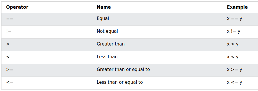
Logical operations
5 > 6
## [1] FALSE
5 + 1 == 6 #NOTE: I am using == to check equality!
## [1] TRUE
1234 != 1234
## [1] FALSE
Storing data in variables
Assigning data to a variable
R uses <- to make assignments. This is a pain to type. You could use
= but it will cause confusion later on.
my_variable <- 5
Both <- and = and work in most cases.
x <- 3
x = 3
…but R programmers use <- for assignments.
- Use
<-to create or update variables
score <- 100
- Use
=for function arguments
mean(x = 1:10)
## [1] 5.5
Why it matters
<- always works.
= sometimes doesn’t (e.g., in loops or formulas).
Types of variables
Variables (also called values) come in many types (or classes). The very basic ones are the following:
my_logical <- TRUE
my_character <- 'this is just a piece of text'
my_numeric <- 1.23455
These are very simple data types. We will often used much more complex ones when working with actual data.
Name <- c("Jon", "Bill", "Maria", "Ben", "Tina")
Age <- c(23, 41, 32, 58, 26)
my_data_frame <- data.frame(Name, Age)
R studio shows values and data separately in the Environment window.
However, this is just a visualization used by R studio. You can use
this window to inspect variables!
Note on naming variables
Try to use descriptive names for variables. And try to stick to a naming convention that works for you - preferably one that makes your code easy to read.
i_like_snake_case <- 'snake_case'
otherPeopleUseCamelCase <- 'CamelCase'
some.people.use.periods <- 'periods.are.allowed'
And_aFew.People_DONTLIKEconventions <- 'Madness, Madness, I tell you!'
From R for Data Science:
There’s an implied contract between you and R: it will do the tedious computation for you, but in return, you must be completely precise in your instructions. Typos matter. Case matters.
Also, it is important that you use names that are not keywords or functions in R. For example, the following is a bad idea:
#length <- 15 ## THIS IS A BAD IDEA
Trick 1: Using the up and down keys
You can use the up and down keys to navigate through the history of commands you’ve entered. This is a very useful feature.
The vector
The vector is another basic variable in R. It’s the simplest type of variable that actually allows you to store something recognizable as ‘data’. We will spend some time on vectors as they are a good place to start to work with relatively simple data. Also, understanding how to work with vectors makes working with more complex data easier. Much of the operations you can do on vectors, which are 1D, can also be done on 2D data frames.
Creating a vector manually
a_vector <- c(1, 5, 4, 9, 0) # Technically an atomic vector
another_one <- c(1, 5.4, TRUE, "hello") # Technically, this is a list
Creating a vector using the : operator
x <- 1:7
y <- 2:-2
Using seq to make a vector
step_size <- seq(1, 10, by=0.25)
length_specified <- seq(1, 10, length.out = 20)
Indexing vectors
Every item in a vector has an index. Vector indices in R start from 1, unlike most programming languages where index start from 0.
my_longer_vector <- c(1, 2, 'three', '4', 'V', 6, 7, 8)
You can use the [] to select (multiple) elements from a vector.
my_single_element <- my_longer_vector[5]
the_start <- my_longer_vector[1:3]
my_part_of_vector <- my_longer_vector[c(1, 2, 5)] # I'm using a vector to select parts of a vector. Life is funny.
You can also use [] to overwrite a part of a vector
my_longer_vector[1:3] <- c('replace', 'this', 'now')
Logical vectors
vector1 <- c(1,5,6,7,2,3,5,4,6,8,1,9,0,1)
binary_vector <- vector1 > 5
binary_vector
##  [1] FALSE FALSE  TRUE  TRUE FALSE FALSE FALSE FALSE  TRUE  TRUE FALSE  TRUE
## [13] FALSE FALSE
some_other_vector <- seq(from = 0, to = 100, length.out = length(vector1))
selected <- some_other_vector[binary_vector]
selected
## [1] 15.38462 23.07692 61.53846 69.23077 84.61538
Another trick
Before we go on, I want to share a simple trick. Using an IDE like Rstudio makes life easier (or at least it should). One of the benefits of the IDE is tab-completion.
[DEMO GOES HERE]
Functions
Now we know how to store data, we can start manipulating the data using functions.
Functions take 0 or more inputs (also called arguments), perform some operation (i.e., the function of the function), and return some output. This output can be complex and consist of multiple parts. These are generic ways in which functions are used:
output <- function_name(arg1 = val1, arg2 = val2, ...)
output <- function_name(val1, val2, ...)
We’ve already encountered a function:
output<-seq(from = 1, to= 123, by = 0.123)
How do we know which arguments a function can take? Using the help:
?seq
Some very simple functions that might be useful.
a <- max(output)
b <- mean(output)
c <- min(output)
d <- ceiling(output)
e <- sd(output)
Here is a function which returns more complex data. At this point, you’re not supposed to know what this function does (it fits a regression line). The point is that it returns complex data with multiple fields.
x <- runif(100)
y <- 10 + 5 * x + rnorm(100)
result <- lm(y ~ x)
print(result)
##
## Call:
## lm(formula = y ~ x)
##
## Coefficients:
## (Intercept)            x
##      10.059        5.094
Getting Help
Built-in Help
R has built-in help. Learning how to use it will save you some frustration.
You can use ?function_name to get help on a specific function. For
example, here we get some help on the lm() function, a function to fit
linear models. We will be using this function a lot.
?lm
or
help(lm)
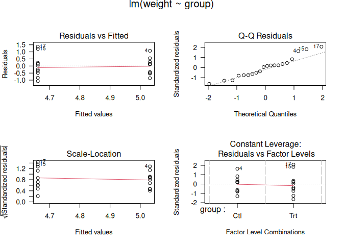
You can also get an example of how to use a function using
example(function_name).
example(lm)
##
## lm> require(graphics)
##
## lm> ## Annette Dobson (1990) "An Introduction to Generalized Linear Models".
## lm> ## Page 9: Plant Weight Data.
## lm> ctl <- c(4.17,5.58,5.18,6.11,4.50,4.61,5.17,4.53,5.33,5.14)
##
## lm> trt <- c(4.81,4.17,4.41,3.59,5.87,3.83,6.03,4.89,4.32,4.69)
##
## lm> group <- gl(2, 10, 20, labels = c("Ctl","Trt"))
##
## lm> weight <- c(ctl, trt)
##
## lm> lm.D9 <- lm(weight ~ group)
##
## lm> lm.D90 <- lm(weight ~ group - 1) # omitting intercept
##
## lm> ## No test:
## lm> ##D anova(lm.D9)
## lm> ##D summary(lm.D90)
## lm> ## End(No test)
## lm> opar <- par(mfrow = c(2,2), oma = c(0, 0, 1.1, 0))
##
## lm> plot(lm.D9, las = 1)      # Residuals, Fitted, ...
##
## lm> par(opar)
##
## lm> ## Don't show:
## lm> ## model frame :
## lm> stopifnot(identical(lm(weight ~ group, method = "model.frame"),
## lm+                     model.frame(lm.D9)))
##
## lm> ## End(Don't show)
## lm> ### less simple examples in "See Also" above
## lm>
## lm>
## lm>
You can also search help pages:
??"linear model"
help.search("regression")
The Internet
The R help system is powerful, but most R users also rely on the Internet for quick answers. It’s important to search with context**
- Combine the task and the tool in your search terms:
r how to merge data frames dply
r plot regression line ggplot2
r error object not found`.
Add the word “r” or the package name to every query — otherwise
you may get unrelated results. Unfortunately, R is a non-descript name
for a programming language.
AI tools
I encourage you to use AI tools but remember you are in charge and responsible for the correctness of your own code.
Give AI tools enough context to work with. For example, instead of just giving the error to an AI tool, copy your code and ask what causes the error.
myata <- data.frame(age = 1:5, score = c(2, 3, 5, 7, 11))
lm(score ~ age, data = mydata)
## Error in eval(mf, parent.frame()): object 'mydata' not found
Tip from the field What I sometimes do is to have AI check my full script (even when I think it works). This sometimes flags up suspicious code that I might want to double-check. It’s an extra pair of eyes to check the code. Below is a very simple example of something that could go wrong. The R parser will see no problems. But AI might flag it up as suspicious.
y <- c(2,3,5,7,11)
X1 <- c(1,2,3,4,5)
X2 <- c(2,6,4,9,15)
X3 <- c(5,3,6,2,1)
model <- lm(y~X1 + X2)
summary(model)
##
## Call:
## lm(formula = y ~ X1 + X2)
##
## Residuals:
##       1       2       3       4       5
##  0.6524 -0.8182  0.1872 -0.5294  0.5080
##
## Coefficients:
##             Estimate Std. Error t value Pr(>|t|)
## (Intercept)  -0.6310     1.0090  -0.625    0.596
## X1            1.4866     0.6772   2.195    0.159
## X2            0.2460     0.2112   1.165    0.364
##
## Residual standard error: 0.9134 on 2 degrees of freedom
## Multiple R-squared:  0.9674, Adjusted R-squared:  0.9348
## F-statistic: 29.69 on 2 and 2 DF,  p-value: 0.03259

> **AI:**
> The model fits fine, but I notice you created `X3` and didn’t include it in the formula.
> If that’s intentional, great — but if you meant to test its effect, update the model to:
> ```r
> model <- lm(y ~ X1 + X2 + X3)
> ```
> Small oversights like unused variables are easy to miss, and an automated code review can help catch them.
Flow control in R
You could write all R scripts as a serial statements of functions. However, to fully exploit the power of programming, you would need to learn about flow control. Flow control refers to (1) executing bits of code depending on a condition, and (2) iteratively executing pieces of code.
This is another introduction to flow control.
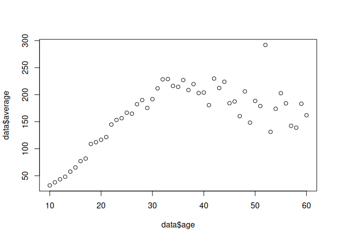
This is a short script which does one thing after another.
data <- read.csv('data/wages1833.csv')
data$average <- ((data$mnum * data$mwage) + (data$fnum * data$fwage)) / (data$mnum + data$fnum)
model <- lm(data$average ~ data$age)
result <- summary(model)
plot(data$age, data$average )
Overview
| Keyword | Use | Example 1 | Example 2 |
|---|---|---|---|
| if (or, else if) | Execute some steps if a condition is true (or false) | If the value of a variable is larger than 5, print it to the screen. | If the result of a statistical test is significant, add a symbol to the graph. |
| For | Repeat some steps for each item in collection, such as a vector. | For each value in a vector, print the value to the screen. | Repeat something exactly n times. |
| While | Repeat some steps as long as something is true (or false). | As long as the value of a variable is smaller than 5, generate a new value for it. | While your data has outliers, remove them.
|
The if statement
This is the basic anatomy of an if statement
if (expression) {
   #statement to execute if condition is true
}
Example:
my_number <-12

if (my_number < 20){
  x <- sprintf('%i is less than 20', my_number)
  print(x)
}
## [1] "12 is less than 20"
The if else statement
There is also an if-else variant of this,
a  <- -5

# condition
if(a > 0)
{
    print("Positive Number")
}else{
    print("negative number")
}
## [1] "negative number"
Rewriting the previous one on 1 line (maybe that makes it easier to read?)
a  <- -5

# condition
if(a > 0){print("Positive Number")}else{print("negative number")}
## [1] "negative number"
The else if statement
a <- 200
b <- 33

if (b > a) {
  print("b is greater than a")
} else if (a == b) {
  print("a and b are equal")
} else {
  print("a is greater than b")
}
## [1] "a is greater than b"
Overview of if statements
ifStatement: use it to execute a block of code, if a specified condition is trueelseStatement: use it to execute a block of code, if the same condition is falseelse ifStatement: use it to specify a new condition to test, if the first condition is
The for loop
The for loop iterates over a sequence.
my_vector <- runif(5)
for (x in my_vector) {
  y <- x * 3
  print(y)
}
## [1] 2.878933
## [1] 2.901794
## [1] 0.3190982
## [1] 2.585775
## [1] 2.924298
Just to drive the point home, another example:
fruits <- list("apple", "banana", "cherry")
for (x in fruits) {
  print(x)
}
## [1] "apple"
## [1] "banana"
## [1] "cherry"
One very common use of the for loop is to iterate a bit of code
exactly n times.
number_of_time_i_want_to_repeat_this <-10
for (x in 1:10) {
  print('This is being repeated!')
}
## [1] "This is being repeated!"
## [1] "This is being repeated!"
## [1] "This is being repeated!"
## [1] "This is being repeated!"
## [1] "This is being repeated!"
## [1] "This is being repeated!"
## [1] "This is being repeated!"
## [1] "This is being repeated!"
## [1] "This is being repeated!"
## [1] "This is being repeated!"
You can use a break statement to break the loop at any point.
number_of_time_i_want_to_repeat_this <-10
for (x in 1:10) {
  print('This is being repeated!')
  if (x > 7){
    print('I quit!')
    break
  }
}
## [1] "This is being repeated!"
## [1] "This is being repeated!"
## [1] "This is being repeated!"
## [1] "This is being repeated!"
## [1] "This is being repeated!"
## [1] "This is being repeated!"
## [1] "This is being repeated!"
## [1] "This is being repeated!"
## [1] "I quit!"
The while loop
The while repeats a piece of code if something is true and as long as it is true.
i <- 1
while (i < 6) {
  print(i)
  i <- i + 1
}
## [1] 1
## [1] 2
## [1] 3
## [1] 4
## [1] 5
The break keyword
You can use break to exit a loop at any time
i <- 1
while (i < 100000) {
  print(i)
  i <- i + 1
  if (i > 5){break}
}
## [1] 1
## [1] 2
## [1] 3
## [1] 4
## [1] 5
Exercises: Flow control
- Write a for loop that iterates over the numbers 1 to 7 and prints the
cube of each number using
print(). - Write a while loop that prints out standard random normal numbers (use
rnorm()) but stops (breaks) if you get a number bigger than 1. - Using a for loop simulate the flip a coin twenty times, keeping track of the individual outcomes (1 = heads, 0 = tails) in a vector.
- Use a while loop to investigate the number of terms required before the series $1 \times 2 \times 3 \times ,\ldots$ reaches above 10 million.
Solutions
One
Write a for loop that iterates over the numbers 1 to 7 and prints the cube of each number using print().
for(i in 1:7){
  print(i^2)
  }
## [1] 1
## [1] 4
## [1] 9
## [1] 16
## [1] 25
## [1] 36
## [1] 49
Two
Write a while loop that prints out standard random normal numbers (use rnorm()) but stops (breaks) if you get a number bigger than 1.
Option 1
value <- 0
counter <-0
while(value < 1)
{
  value <- rnorm(1)
  counter <- counter + 1
}
print(value)
## [1] 1.954834
print(counter)
## [1] 5
Option 2
counter <-0
while(TRUE)
{
  value <- rnorm(1)
  counter <- counter + 1
  if (value > 1){break}
}
print(value)
## [1] 1.362865
print(counter)
## [1] 10
Three
Using a for loop simulate the flip a coin twenty times, keeping track of the individual outcomes (1 = heads, 0 = tails) in a vector.
repeats <- 20
outcomes <- character(repeats)
for(i in 1:repeats)
{
  outcome <- sample(c('H','T'), 1)
  outcomes[i] <- outcome
}
outcomes
##  [1] "H" "H" "H" "T" "T" "H" "T" "T" "H" "T" "T" "H" "T" "H" "H" "T" "T" "H" "T"
## [20] "H"
You could do this in one line (but that was not the exercise).
repeats <- 20
outcomes <- sample(c('H','T'), repeats, replace = TRUE)
outcomes
##  [1] "H" "H" "H" "T" "T" "T" "T" "T" "T" "H" "T" "T" "H" "T" "T" "T" "T" "H" "H"
## [20] "T"
Four
Use a while loop to investigate the number of terms required before the series 1 ,reaches above 10 million.
product <- 1
term <- 0

while(product < 10000000)
{
  term <- term + 1
  product <- product * term

}
print(term)
## [1] 11
# Check
1:term
## [1] 1 2 3 4 5 6 7 8 9 10 11
cumprod(1:term)>10000000
## [1] FALSE FALSE FALSE FALSE FALSE FALSE FALSE FALSE FALSE FALSE TRUE
Note on vector preallocation
This piece of code builds a vector by appending numbers to the end of it.
repeats <- 10000
startTime <- Sys.time()
my_vector <- c()
for (i in 0:repeats){
  x <- runif(1)
  vector <- append(vector, x)
}
endTime <- Sys.time()
print(sprintf('Duration: %.2f', endTime - startTime))
## [1] "Duration: 0.43"
This piece of code preallocates a vector and is more efficient.
repeats <- 10000
startTime <- Sys.time()
my_vector <- numeric(repeats)
for (i in 0:repeats){
  x <- runif(1)
  vector[i] <- x
  }
endTime <- Sys.time()
print(sprintf('Duration: %.2f', endTime - startTime))
## [1] "Duration: 0.03"
Working with text: the paste() function
x <- runif(100)
y <- 10 + 5 * x + rnorm(100)
result <- lm(y ~ x)
summary(result)
##
## Call:
## lm(formula = y ~ x)
##
## Residuals:
##     Min      1Q  Median      3Q     Max
## -2.4195 -0.7328 -0.0227  0.6718  3.4195
##
## Coefficients:
##             Estimate Std. Error t value Pr(>|t|)
## (Intercept)  10.0538     0.1936   51.94   <2e-16 ***
## x             4.9407     0.3546   13.93   <2e-16 ***
## ---
## Signif. codes:  0 '***' 0.001 '**' 0.01 '*' 0.05 '.' 0.1 ' ' 1
##
## Residual standard error: 1.017 on 98 degrees of freedom
## Multiple R-squared:  0.6645, Adjusted R-squared:  0.6611
## F-statistic: 194.1 on 1 and 98 DF,  p-value: < 2.2e-16
test1 <- paste(10000)
test2<-paste(result$coefficients[1], result$coefficients[2], sep = ', ')
test3<-paste('The coefficients are: ', result$coefficients[1],  ', ', result$coefficients[2], sep='')
print(test1)
## [1] "10000"
print(test2)
## [1] "10.0538038862781, 4.94070059507232"
print(test3)
## [1] "The coefficients are: 10.0538038862781, 4.94070059507232"
for (x in 1:10) {print(test3)}
## [1] "The coefficients are: 10.0538038862781, 4.94070059507232"
## [1] "The coefficients are: 10.0538038862781, 4.94070059507232"
## [1] "The coefficients are: 10.0538038862781, 4.94070059507232"
## [1] "The coefficients are: 10.0538038862781, 4.94070059507232"
## [1] "The coefficients are: 10.0538038862781, 4.94070059507232"
## [1] "The coefficients are: 10.0538038862781, 4.94070059507232"
## [1] "The coefficients are: 10.0538038862781, 4.94070059507232"
## [1] "The coefficients are: 10.0538038862781, 4.94070059507232"
## [1] "The coefficients are: 10.0538038862781, 4.94070059507232"
## [1] "The coefficients are: 10.0538038862781, 4.94070059507232"
Session info (Tech details)
sessionInfo()
## R version 4.3.3 (2024-02-29)
## Platform: x86_64-pc-linux-gnu (64-bit)
## Running under: Linux Mint 22.2
##
## Matrix products: default
## BLAS:   /usr/lib/x86_64-linux-gnu/openblas-pthread/libblas.so.3
## LAPACK: /usr/lib/x86_64-linux-gnu/openblas-pthread/libopenblasp-r0.3.26.so;  LAPACK version 3.12.0
##
## locale:
##  [1] LC_CTYPE=en_US.UTF-8       LC_NUMERIC=C
##  [3] LC_TIME=en_US.UTF-8        LC_COLLATE=en_US.UTF-8
##  [5] LC_MONETARY=en_US.UTF-8    LC_MESSAGES=en_US.UTF-8
##  [7] LC_PAPER=en_US.UTF-8       LC_NAME=C
##  [9] LC_ADDRESS=C               LC_TELEPHONE=C
## [11] LC_MEASUREMENT=en_US.UTF-8 LC_IDENTIFICATION=C
##
## time zone: America/New_York
## tzcode source: system (glibc)
##
## attached base packages:
## [1] stats     graphics  grDevices utils     datasets  methods   base
##
## loaded via a namespace (and not attached):
##  [1] compiler_4.3.3    fastmap_1.2.0     cli_3.6.5         tools_4.3.3
##  [5] htmltools_0.5.8.1 yaml_2.3.10       rmarkdown_2.30    knitr_1.50
##  [9] xfun_0.53         digest_0.6.37     rlang_1.1.6       evaluate_1.0.5